
Example Numpy calculation
For the following, we will often use normal Numpy as a baseline. Remember it's already a factor of 10 to 100 faster than pure Python!
Let's pretend that we have the following calculation, and it's important to us for some reason:
$$ y = x + x^2 + x^3 + x^4 + x^5 + x^6 + x^7 + x^8 $$import numpy as np
from scipy.stats import norm
import matplotlib.pyplot as plt
import numexpr
import numba
For all the following examples, we'll use the same 1M element vector:
x = np.random.normal(size=1_000_000)
def f_simple(xarr):
    yarr = np.empty_like(xarr)
    for i in range(len(xarr)):
        x = xarr[i]
        yarr[i] = x + x**2 + x**3 + x**4 + x**5 + x**6 + x**7 + x**8
    return yarr
%%timeit
f_simple(x)
def f_numpy(x):
    return x + x**2 + x**3 + x**4 + x**5 + x**6 + x**7 + x**8
%%timeit
f_numpy(x)
Note that this is clean and clear. If this is fast enough for your use case, stop here! This is the easiest one to maintain, and is the most similar to the original problem statement.
It is slow, however, We have to make a lot of memory allocations; even though we can reclaim it later, this is slow. Also, raising to a power is a bit pricey too.
def f_nest_numpy(x):
    return x*(1 + x*(1 + x*(1 + x*(1 + x*(1 + x*(1 + x*(1 + x)))))))
np.testing.assert_allclose(f_numpy(x), f_nest_numpy(x))
%%timeit
f_nest_numpy(x)
def f_mem_numpy(x):
    y = x.copy()
    for _ in range(7):
        y += 1
        y *= x
    return y
np.testing.assert_allclose(f_numpy(x), f_mem_numpy(x))
%%timeit
f_mem_numpy(x)
Wow! Almost all the time in the previous examples was memory allocation!
Most of Numpy's functionality can be accessed with pre-allocated memory. You can use the out= keyword argument in many functions to put the results of many function calls directly in existing memory, for example.
However, we can't always get rid of memory allocation, depending on the problem, and we are now much further from the original math expression. Let's see if we can use a library to help.
Numexpr
We can't resist a quick look at the numexpr JIT compiler. It's an oldy but a goody for simple use cases. If you have long, simple numpy expressions, you can put them inside a string, and numexpr will create an optimized version of this without in-between expressions that Python would require, and then evaluate that. Let's see:
def f_numexper(x):
    return numexpr.evaluate('x + x**2 + x**3 + x**4 + x**5 + x**6 + x**7 + x**8')
np.testing.assert_allclose(f_numpy(x), f_numexper(x))
%%timeit
f_numexper(x)
Nice! The downside: It only supports a small handful of operations and functions, like sin and cos. It's also best used for simple bits like this. However, your code is pretty readable (albeit in a string), and if used carefully, could be all you'll need. Numexpr must be available, of course, but it usually is.
Cython: A new language
I can't skip Cython. It revolutionized Python in many ways, though as you'll see soon, I don't think it's the best tool for the job anymore. It allows you to write a mix of Python and C to create completely pre-compiled functions. Compared to writing the Python C-API, it's amazing. Compared to pretty much anything else...
Compiling Cython is often a pain, but it has a Jupyter extension that is excellent, so let's use that.
%load_ext Cython
%%cython
# cython: boundscheck=False, wraparound=False, noncheck=False, cdivision=True

import numpy as np

def f_cython(double[:] xarr):
    y_arr = np.empty([len(xarr)])
    cdef double[:] y = y_arr
    cdef int i
    cdef double x

    for i in range(xarr.shape[0]):
        x = xarr[i]
        y[i] = x*(1 + x*(1 + x*(1 + x*(1 + x*(1 + x*(1 + x*(1 + x)))))))
        #y[i] = x + x**2 + x**3 + x**4 + x**5 + x**6 + x**7 + x**8

    return y
np.testing.assert_allclose(f_numpy(x), f_cython(x))
%%timeit
f_cython(x)
Yes, this is overkill. Even if you know Python, C, and C++, this is still a new language with its own quirks. But it does give you lots of power for complex tasks - you can even write classes! You can activate C++ mode and call existing C++ libraries! Yes, compiling gets exponentially harder to do if you do that, but it's possible. Not pretty, just possible. You can use OpenMP to run in multiple threads, again making the compile step more complicated (I'm not showing that on macOS here!)
Now let's look at the new kid on the scene:
Numba
Numba takes a totally different approach. It's built on two ideas:
- It reads and converts byte code from existing Python functions
- It does JIT compilation directly to LLVM (no C or C++ in-between)
Why is that special or new?
- 100% Python - no special compiler, special extensions, strings, etc.
- Easy to make optional - just don't run the function through Numba - no Numba requirement
- It's a just a library! No new interpreter or compiler step
For now, let's not even bother to write a new function! We have perfectly nice existing functions, let's just pass them through Numba:
f_numba_simple = numba.jit(f_numpy)
f_numba_nest = numba.jit(f_nest_numpy)
np.testing.assert_allclose(f_numpy(x), f_numba_simple(x))
np.testing.assert_allclose(f_nest_numpy(x), f_numba_nest(x))
%%timeit
f_numba_simple(x)
%%timeit
f_numba_nest(x)
Wow! We didn't do anything at all to our original, slow source code. We even reused it! We could have written a check for Numba, and only applied the JIT if Numba was found - free speedup.
f_numba_simple_ufunc = numba.vectorize([numba.double(numba.double)],
                                       target='parallel')(f_numpy)
f_numba_nest_ufunc = numba.vectorize([numba.double(numba.double)],
                                     target='parallel')(f_numba_nest)
np.testing.assert_allclose(f_numpy(x), f_numba_simple_ufunc(x))
np.testing.assert_allclose(f_numpy(x), f_numba_nest_ufunc(x))
%%timeit
f_numba_simple_ufunc(x)
%%timeit
f_numba_nest_ufunc(x)
f_numba_parallel = numba.jit(nopython=True, parallel=True)(f_numpy)
np.testing.assert_allclose(f_numpy(x), f_numba_parallel(x))
%%timeit
f_numba_parallel(x)
jit: Compile a function. Unlike Cython, this supports array-at-a-time syntax.njitisjit(nopython=True)vectorize: Make a UFunc. You write a 1 element function, and it gets applied to all elements.guvectorize: Make a Generalized UFunc. You can specify relations for the input/output shapescfunc: Callable from other Numba routines only (jit functions can be called too)
Lesser used / more specialized / underdeveloped:
jitclass: Write a class instead of a function (early support warning has been there for a long time)stencil: Masking operationsoverload: Make a nopython version of a function- GPU versions: You can target CUDA with
cuda.jit,vectorize(target='cuda')(limited feature set) - You recently can target AMD ROC GPUs too
See the Numba documentation for more. You can find a list of functions and features supported - it's far more extensive than numexpr! (Note that the CUDA and ROC versions have fewer features supported)
Common options (not all are available on all functions):
- A signature or list of signatures: Precompile the function with these expected types
nopython=True: force the function to fail if it can't become a pure Numba compiled functiontarget=: Can be one ofcpu,parallel,gpu,cuda, depending on the functionfastmath=True: Can speed up math at some accuracy costparallel=True: Just onjit, can try to parallelizenogil=True: Release Python's global interpreter lock on memory
Numba is under rapid development, with a new release every 2-3 months. Each release adds features from Intel's collaboration, often a few AMD features now, new supported functions, and lots more.
f_numba_simple.inspect_types()
#print(list(f_numba_simple.inspect_llvm().values())[0])
Real code example
Here is some real code that I've written recently. I had a training sample that took 60 seconds to run an iteration. The original (non-decorated version) took 100+ seconds to run on 10K events. The decorated version, with some small changes to remove list appending, takes <0.1 second and can be run every iteration.
The code looks for signals that look like bumps in an array of mostly zeros following a specific set of requirements (threshold, integral_threshold, min_width).
@numba.jit(numba.float32[:](numba.float32[:], numba.float32, numba.float32, numba.int32),
           locals={'integral':numba.float32, 'sum_weights_locs':numba.float32},
           nopython=True)
def pv_locations(targets, threshold, integral_threshold, min_width):
    state = 0
    integral = 0.0
    sum_weights_locs = 0.0

    # Make an empty array and manually track the size (faster than python array)
    items = np.empty(150, np.float32)
    nitems = 0

    for i in range(len(targets)):
        if targets[i] >= threshold:
            state += 1
            integral += targets[i]
            sum_weights_locs += i * targets[i] # weight times location

        if (targets[i] < threshold or i == len(targets)-1) and state > 0:

            # Record only if
            if state >= min_width and integral >= integral_threshold:
                items[nitems] = sum_weights_locs / integral
                nitems += 1

            #reset state
            state = 0
            integral = 0.0
            sum_weights_locs = 0.0


    # Special case for final item (very rare or never occuring)
    # handled by above if len

    return items[:nitems]
import matplotlib.pyplot as plt
size = (500, 500)
iterations = 50

def make_fractal(size, iterations):
    x = np.linspace(-2,2,size[0]).reshape(1,-1)
    y = np.linspace(-2,2,size[1]).reshape(-1,1)
    c = x + y*1j
    z = np.zeros_like(c)
    it_matrix = np.zeros(size, dtype=np.int)
    for n in range(iterations):
        z = z**2 + c
        it_matrix[np.abs(z) < 2] = n
    return it_matrix
plt.figure(figsize=(10,10))
plt.imshow(make_fractal(size, iterations));
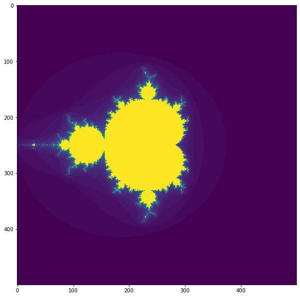
%%timeit
make_fractal(size, iterations)
@numba.jit(nopython=True)
def make_fractal_nb(size, iterations):
    x = np.linspace(-2,2,size[0]).reshape(1,-1)
    y = np.linspace(-2,2,size[1]).reshape(-1,1)
    c = x + y*1j
    z = np.zeros_like(c)
    it_matrix = np.zeros(size, dtype=np.int64)
    for n in range(iterations):
        for i in range(size[0]):
            for j in range(size[1]):
                if np.abs(z[i,j]) < 2:
                    z[i,j] = z[i,j]**2 + c[i,j]
                    it_matrix[i, j] = n
    return it_matrix
plt.figure(figsize=(10,10))
plt.imshow(make_fractal_nb(size, iterations));
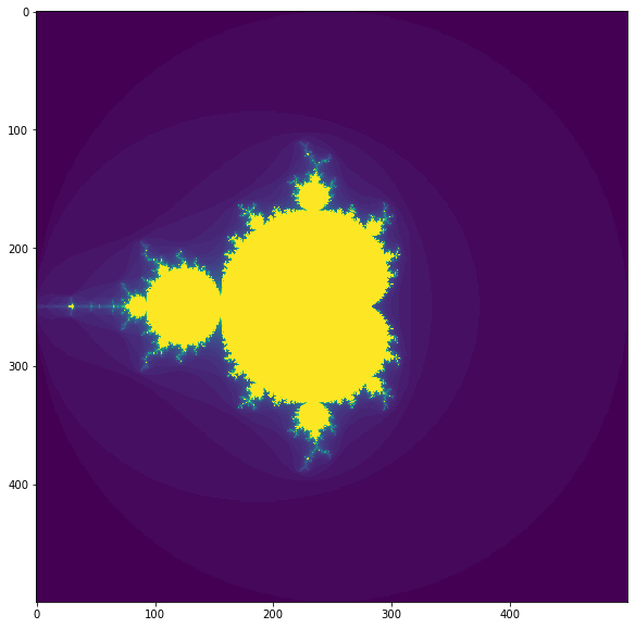
%%timeit
make_fractal_nb(size, iterations)
def sampler(data, samples=4, mu_init=.5, proposal_width=.5, plot=False, mu_prior_mu=0, mu_prior_sd=1.):
    mu_current = mu_init
    posterior = [mu_current]
    for i in range(samples):
        # suggest new position
        mu_proposal = norm(mu_current, proposal_width).rvs()

        # Compute likelihood by multiplying probabilities of each data point
        likelihood_current = norm(mu_current, 1).pdf(data).prod()
        likelihood_proposal = norm(mu_proposal, 1).pdf(data).prod()

        # Compute prior probability of current and proposed mu
        prior_current = norm(mu_prior_mu, mu_prior_sd).pdf(mu_current)
        prior_proposal = norm(mu_prior_mu, mu_prior_sd).pdf(mu_proposal)

        p_current = likelihood_current * prior_current
        p_proposal = likelihood_proposal * prior_proposal

        # Accept proposal?
        p_accept = p_proposal / p_current

        # Usually would include prior probability, which we neglect here for simplicity
        accept = np.random.rand() < p_accept

        if plot:
            plot_proposal(mu_current, mu_proposal, mu_prior_mu, mu_prior_sd, data, accept, posterior, i)

        if accept:
            # Update position
            mu_current = mu_proposal

        posterior.append(mu_current)

    return posterior
%%time
np.random.seed(123)
data = np.random.randn(20)

posterior = sampler(data, samples=1500, mu_init=1.)
Now let's replace the scipy calls, and rerun:
def norm_pdf(loc, scale, x):
    y = (x - loc) / scale
    return np.exp(-y**2/2)/np.sqrt(2*np.pi) / scale
Make sure it's really the same:
assert norm_pdf(.4, .7, .2) == norm(.4, .7).pdf(.2)
assert norm(.3, 1).pdf(data).prod() == np.prod(norm_pdf(.3,1,data))
We'll also remove the list appending.
def sampler(data, samples=4, mu_init=.5, proposal_width=.5, plot=False, mu_prior_mu=0, mu_prior_sd=1.):
    mu_current = mu_init

    posterior = np.empty(samples+1)
    posterior[0] = mu_current

    for i in range(samples):
        # suggest new position
        mu_proposal = np.random.normal(mu_current, proposal_width)

        # Compute likelihood by multiplying probabilities of each data point
        likelihood_current = np.prod(norm_pdf(mu_current, 1, data))
        likelihood_proposal = np.prod(norm_pdf(mu_proposal, 1, data))

        # Compute prior probability of current and proposed mu
        prior_current = norm_pdf(mu_prior_mu, mu_prior_sd, mu_current)
        prior_proposal = norm_pdf(mu_prior_mu, mu_prior_sd, mu_proposal)

        p_current = likelihood_current * prior_current
        p_proposal = likelihood_proposal * prior_proposal

        # Accept proposal?
        p_accept = p_proposal / p_current

        # Usually would include prior probability, which we neglect here for simplicity
        accept = np.random.rand() < p_accept

        if accept:
            # Update position
            mu_current = mu_proposal

        posterior[i+1] = mu_current

    return posterior
%%time
np.random.seed(123)
data = np.random.randn(20)

posterior = sampler(data, samples=1500, mu_init=1.)
Okay, instanciating scipy distributions over and over again is very costly....
@numba.jit
def norm_pdf(loc, scale, x):
    y = (x - loc) / scale
    return np.exp(-y**2/2)/np.sqrt(2*np.pi) / scale
@numba.jit(nopython=True)
def sampler(data, samples=4, mu_init=.5, proposal_width=.5, plot=False, mu_prior_mu=0, mu_prior_sd=1.):
    mu_current = mu_init

    posterior = np.empty(samples+1)
    posterior[0] = mu_current

    for i in range(samples):
        # suggest new position
        mu_proposal = np.random.normal(mu_current, proposal_width)

        # Compute likelihood by multiplying probabilities of each data point
        likelihood_current = np.prod(norm_pdf(mu_current, 1, data))
        likelihood_proposal = np.prod(norm_pdf(mu_proposal, 1, data))

        # Compute prior probability of current and proposed mu
        prior_current = norm_pdf(mu_prior_mu, mu_prior_sd, mu_current)
        prior_proposal = norm_pdf(mu_prior_mu, mu_prior_sd, mu_proposal)

        p_current = likelihood_current * prior_current
        p_proposal = likelihood_proposal * prior_proposal

        # Accept proposal?
        p_accept = p_proposal / p_current

        # Usually would include prior probability, which we neglect here for simplicity
        accept = np.random.rand() < p_accept

        if accept:
            # Update position
            mu_current = mu_proposal

        posterior[i+1] = mu_current

    return posterior
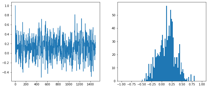
fig, axs = plt.subplots(1,2, figsize=(12,5))
vals = sampler(data, samples=1500, mu_init=1.)
axs[0].plot(vals)
axs[1].hist(vals[500:], bins=np.linspace(-1,1,100))
plt.show()
%%time
np.random.seed(123)
data = np.random.randn(20)

posterior = sampler(data, samples=1500, mu_init=1.)