Numerical tools
Objectives
- Learn how to use numpy's arrays
- Learn how to maninipulate arrays without loops
- Learn about broadcasting
See https://docs.scipy.org/doc/numpy/user/quickstart.html for similar material.
(a,) = [1]
c, d = [1, 2]
begin, *middle, end = range(5)
print(a)
print(begin)
print(middle)
Numpy arrays are iterable, so we'll use this a few times in the upcoming material. You may also have seen it in my tests, since it's a handy way to get values from an iterable while also enforcing the length. This is also the basis for the swap idiom in Python:
c, d = d, c
import numpy as np
Arrays
The numpy library is build around the array. Arrays are different from Python lists:
- Arrays can be multidimensional, and have a
.shape - Arrays hold a specific data type (called
dtype) only - Arrays cannot change size inplace (but can change shape)
- Operations are element-wise
If you have used Matlab before, note that arrays in Python support 0 and 1 dimensions besides the normal 2+, and that operations are elementwise.
Arrays can be created from lists and tuples (not all iterables, though - Numpy looks explicitly for nested lists and tuples to make multiple dimensions)
arr = np.array([1, 2, 3, 4])
arr
The shape of an array is a tuple, with one element per dimension
arr.shape
You can also access the dtype (type of the data):
arr.dtype
Numpy tries to pick the best dtype based on your input data; it will pick int if there are no floats:
print(np.array([1, 1]).dtype)
print(np.array([1, 1.0]).dtype)
print(np.array([1, 1], dtype=np.float64).dtype)
The good news: dtype is automatically upgraded if needed unless you are doing in-place operations
Operations on an array are defined as elementwise (with the exceptions of the logic operators - numpy uses bitwise operators instead).
arr ** 2
If you want to use logic operators, use the bitwise operators instead, and lots of parenthesis:
(arr == 1) | (arr == 2)
np.zeros(3)
np.zeros(3, dtype=np.int8)
np.ones([2, 2])
Multidiminsional arrays are supported, too. (If you know about array ordering, Numpy defaults to C order, and can do Fortran order also)
np.eye(3)
np.random.rand(2, 2)
np.random.randint(2, 5, (3, 4))
Ufuncs
Numpy also provides UFuncs; functions that apply element-wise to an array. They do so without a Python loop, making them very fast. There are also a collection of other useful functions that do things like sum without Python loops.
Technically, UFuncs must produce the same size output array. Ones that produce different output array sizes are called Generalized UFuncs, but that distinction will not matter to us for now.
np.sin(arr)
np.exp(arr)
np.sum(arr)
a = np.eye(4)
a
a.reshape(2, 8)
a.reshape(2, -1)
a.reshape(1, 16)
a.reshape(16)
a.flatten()
We can also add new empty axis:
b = np.array([1, 2, 3])
b[:, np.newaxis]
b[np.newaxis, :]
np.uint8(1)
np.float16(12.123456789123456789123456789)
arr = np.arange(16).reshape(4, 4)
arr
Unlike matlab, a single index returns a row (or the remaining N-1 dimensions):
arr[0]
You could nest calls (arr[0][0]), but Numpy uses Python's rich index support to make this simpler and faster:
arr[0, 0]
Slices are supported:
arr[:, 0]
Just like normal Python, a slice retains a dimension, while a single number does not.
Unless you work with large numbers of dimensions, this probably won't be useful, but ... means "all the remaining dimensions":
- This is rarely used
- This was actually added to Python at Numpy's request
- This may be the only time in the course I get to use the
...for what it was intended for!
arr[..., 0]
Boolean arrays also can index! (You can also uses lists, like I am doing in this example - but usually you will use a np.array, and it does not work with tuples)
np.arange(4)[[True, False, True, False]]
More realistic example: (note that due to the selection, output is always 1D)
arr[arr < 8]
Remember that arr[...] = was one of the (few) allowed assignment expressions!
arr[arr < 8] = 1
arr
Remember I told you assignment operations were special? What do you think this might do? And why did I try adding the [:]?
b = arr[arr < 8]
b[:] = 2
arr
The expression a[...] = b turns into
a.__setitem__(..., b)
While a = b unceremoniously replaces b, no methods called. And, for b = a[...], a.__getitem__(...) is called.
Note for the curious: the stuff in the
...part gets turned into a tuple, unless it already is one. This is why tuples behave different than lists in indexing.
</font>
a = np.arange(4).reshape(2, 2)
b = np.array([1, 2])[:, np.newaxis]
print(a)
print(b)
print(a * b)
Suggestion: don't try to mix arrays that don't have matching dimension: broadcasting is not clear in intent there. The one exception: scalars (0D)
a + 2
x, y = np.mgrid[:3, :3]
# np.meshgrid(np.arange(3), np.arange(3))
x * 2 + y
x, y = np.ogrid[:3, :3]
x * 2 + y
import matplotlib.pyplot as plt
import numpy as np
# Size of the grid to evaluate on
size = (500, 500)
xs = np.linspace(-2, 2, size[0])
ys = np.linspace(-2, 2, size[1])
# We need to make a grid where values x = real and y = imag
x, y = np.meshgrid(xs, ys)
# We could also write: x, y = np.mgrid[-2:2:100j, -2:2:100j]
# Or use open grids and broadcasting
c = x + y * 1j
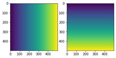
# Verify that we have correctly constructed the real and imaginary parts
fig, axs = plt.subplots(1, 2)
axs[0].imshow(c.real)
axs[1].imshow(c.imag)
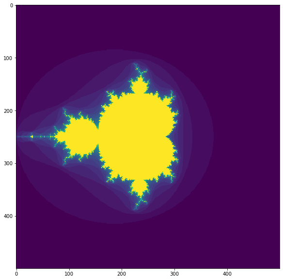
z = np.zeros(size, dtype=np.complex)
it_matrix = np.zeros(size, dtype=np.int)
for n in range(30):
    z = z ** 2 + c
    it_matrix[np.abs(z) < 2] = n
plt.figure(figsize=(10, 10))
plt.imshow(it_matrix)
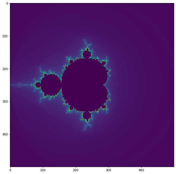
z = np.zeros(size, dtype=np.complex)
it_matrix = np.zeros(size, dtype=np.double)
for n in range(50):
    z[it_matrix == 0] = z[it_matrix == 0] ** 2 + c[it_matrix == 0]
    filt = (it_matrix == 0) & (np.abs(z) > 2)
    it_matrix[filt] = n + 1 - np.log(np.log(np.abs(z[filt]))) / np.log(2)
plt.figure(figsize=(10, 10))
plt.imshow(it_matrix)
Try it yourself:
- Put together a function that computes the mandelbrot set. Make at least the size a default parameter.
- Adjust parameters to see the effect
See also https://www.ibm.com/developerworks/community/blogs/jfp/entry/How_To_Compute_Mandelbrodt_Set_Quickly?lang=en for way too many ways to do mandelbrots in Python, along with performance measurements.


