import numpy as np
import matplotlib.pyplot as plt
def f_diff(f, x, h):
    """
    Forward difference method.
    f is a function,
    x is the point(s),
    h is the distance to use for the difference.
    """
    return (f(x + h) - f(x)) / h
Let's compare a known derivative and a numerical one:
np.cos(1)
f_diff(np.sin, 1, 1e-5)
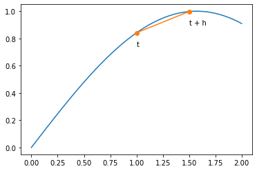
x = np.linspace(0, 2)
tth = np.array([1, 1.5])
plt.plot(x, np.sin(x))  # The f(x) (blue) curve
plt.plot(tth, np.sin(tth), "o-")  # The straight line
plt.text(tth[0], np.sin(tth[0]) - 0.1, "t")
plt.text(tth[1], np.sin(tth[1]) - 0.1, "t + h")
plt.show()
This is a simple formula if you simply take very small $h$, but it has a problem: We are subtracting nearly identical values. This is exactly what we said was bad for numerical precision!
How do we choose an ideal $h$? We'll come back to this soon. Let's cover a slight modification of the last formula first, though.
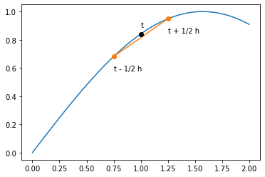
x = np.linspace(0, 2)
tth = np.array([1 - 0.25, 1 + 0.25])
plt.plot(x, np.sin(x))  # The f(x) (blue) curve
plt.plot(tth, np.sin(tth), "o-")  # The straight line
plt.plot(1, np.sin(1), "ko")  # A black ('k') dot
plt.text(1, np.sin(1) + 0.05, "t")
plt.text(tth[0], np.sin(tth[0]) - 0.1, "t - 1/2 h")
plt.text(tth[1], np.sin(tth[1]) - 0.1, "t + 1/2 h")
plt.show()
def c_diff(f, x, h):
    """
    Central difference method.
    f is a function,
    x is the point(s),
    h is the distance to use for the difference.
    """
    return (f(x + h / 2) - f(x - h / 2)) / h
h = 1e-5
print(c_diff(np.sin, 1, h), "- centeral")
print(np.cos(1), "- true")
print(f_diff(np.sin, 1, h), "- forward")
Extrapolated difference
We can combine wider an narrower steps to do even better for a smooth function, though with the downside that we are now evaluating the function at more points.
$$ \frac{dy(t)}{dt} \Biggr\rvert_\mathrm{ed} = \frac{ 4 D_\mathrm{cd}(t, h/2) - D_\mathrm{cd}(t, h/2) }{3} \tag{4} $$def ex_diff(f, x, h):
"""
Extended difference method.
f is a function,
x is the point(s),
h is the distance to use for the difference.
"""
return (4 * c_diff(f, x, h / 2) - c_diff(f, x, h)) / 3
h = 1e-5
print(c_diff(np.sin, 1, h), "- centeral")
print(np.cos(1), "- true")
print(ex_diff(np.sin, 1, h), "- extended")
Second derivatives
$$ \frac{d^2 f(t)}{dt^2} \Biggr\rvert_\mathrm{cd} = \frac{f(t + h) + f(t - h) - 2 f(t)}{h^2} \tag{5} $$$$ = \frac{ \left[ f(t + h) - f(t) \right] - \left[ f(t) - f(t - h) \right] }{h^2} \tag{6} $$While (5) looks nicer, (6) is computationally better (as long as you are thoughtful about function calls if that matters for you).
- Homework 5: You'll be asked to write a function that calculates the second derivative.
def f1(V, x):
    "The left side of the energy equation"
    return np.sqrt(V - x) * np.tan(np.sqrt(V - x))


def f2(x):
    "The right side of the energy equation"
    return np.sqrt(x)


def sub_f12(V, x):
    "One minus the other should be 0, we'll search for 0s."
    return f1(V, x) - f2(x)
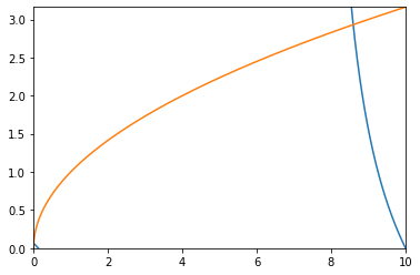
Let's plot both sides of that equation:
V = 10
x = np.linspace(0, V, 1000)
y1 = f1(V, x)
y1 = np.ma.masked_array(y1, y1 < 0)
plt.plot(x, y1)
plt.plot(x, f2(x))
plt.ylim(0, np.max(f2(x)))
plt.xlim(0, V)
plt.show()
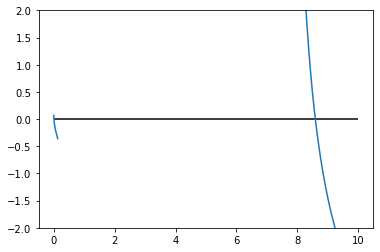
Now, let's plot the left side minus the right side:
y = sub_f12(V, x)
y = np.ma.masked_array(y, y1 < 0)
plt.plot(x, y)
plt.ylim(-2, 2)
plt.hlines(0, 0, V)
plt.show()
search = np.array([0, 0.2])  # Must be floating point

for i in range(20):
    vmid = np.mean(search)  # midway between the points
    fmid = sub_f12(V, vmid)  # function eval

    # Check to see if the sign of the first point
    # is the same as our midpoint
    if np.sign(fmid) == np.sign(sub_f12(V, search[0])):
        search[0] = vmid
    else:
        search[1] = vmid
    print(f"{search[0]:11.5} {search[1]:11.5} {fmid:11.5}")
Aside: setting function parameters
We made a "mistake" with our function definition. We have a function $f(V,x)$, but our functions that take derivatives all expect $f(x)$! It turns out we can use functools.partial to make a new function with some of the function parameters already set. (This is called "currying" in some languages).
from functools import partial

# Before: sub_f12(V,x)
sub_f12_V = partial(sub_f12, V)
# After: sub_f12_V(x)
Okay, ready to find the same 0 as before:
guess = 0

for i in range(10):
    dfdx = f_diff(sub_f12_V, guess, 0.00001)
    fval = sub_f12_V(guess)  # Function at old guess
    guess -= fval / dfdx  # Update guess
    fval = sub_f12_V(guess)  # Function at new guess
    print(f"{guess:11.5} {fval:11.5}")


