import numpy as np
import matplotlib.pyplot as plt
We can rewrite our harmonic motion equation in terms of $\mathbf{f}(t, \mathbf{y}) = \dot{\mathbf{y}}$, where this is in the standard form:
$$ \mathbf{y} = \left( \begin{matrix} \dot{x} \\ x \end{matrix} \right) $$$$ \mathbf{f}(t, \mathbf{y}) = \dot{\mathbf{y}} = \left( \begin{matrix} \ddot{x} \\ \dot{x} \end{matrix} \right) = \left( \begin{matrix} -\frac{k}{m} x \\ \dot{x} \end{matrix} \right) = \left( \begin{matrix} -\frac{k}{m} y_1 \\ y_0 \end{matrix} \right) $$x_max = 1 # Size of x max
v_0 = 0
koverm = 1 # k / m
def f(t, y):
"Y has two elements, x and v"
return np.array([-koverm * y[1], y[0]])
def euler_ivp(f, init_y, t):
    steps = len(t)
    order = len(init_y)  # Number of equations

    y = np.empty((steps, order))
    y[0] = init_y  # Note that this sets the elements of the first row

    for n in range(steps - 1):
        h = t[n + 1] - t[n]

        # Copute dydt based on *current* position
        dydt = f(t[n], y[n])

        # Compute next velocity and position
        y[n + 1] = y[n] - dydt * h

    return y
ts = np.linspace(0, 40, 1000 + 1)
y = euler_ivp(f, [x_max, v_0], ts)
plt.plot(ts, np.cos(ts))
plt.plot(ts, y[:, 0], "--")
Now, expand $f$ in a Taylor series around the midpoint of the interval:
$$ f(t,y) \approx f(t_{n+\frac{1}{2}},y_{n+\frac{1}{2}}) + \left( t - t_{n+\frac{1}{2}}\right) \dot{f}(t_{n+\frac{1}{2}}) + \mathcal{O}(h^2) $$The second term here is symmetric in the interval, so all we have left is the first term in the integral:
$$ \int_{t_n}^{t_{n+1}} f(t,y) \, dt \approx h\, f(t_{n+\frac{1}{2}},y_{n+\frac{1}{2}}) + \mathcal{O}(h^3) $$Back into the original statement, we get:
$$ y_{n+1} \approx \color{blue}{ y_{n} + h\, f(t_{n+\frac{1}{2}},y_{n+\frac{1}{2}}) } + \mathcal{O}(h^3) \tag{rk2} $$We've got one more problem! How do we calculate $f(t_{n+\frac{1}{2}},y_{n+\frac{1}{2}})$? We can use the Euler's algorithm that we saw last time:
$$ y_{n+\frac{1}{2}} \approx y_n + \frac{1}{2} h \dot{y} = \color{red}{ y_n + \frac{1}{2} h f(t_{n},y_{n}) } $$Putting it together, this is our RK2 algorithm:
$$ \mathbf{y}_{n+1} \approx \color{blue}{ \mathbf{y}_{n} + \mathbf{k}_2 } \tag{1.0} $$$$ \mathbf{k}_1 = h \mathbf{f}(t_n,\, \mathbf{y}_n) \tag{1.1} $$$$ \mathbf{k}_2 = h \mathbf{f}(t_n + \frac{h}{2},\, \color{red}{\mathbf{y}_n + \frac{\mathbf{k}_1}{2}}) \tag{1.2} $$Like the book, we've picked up bold face to indicate that we can have a vector of ODEs.
def rk2_ivp(f, init_y, t):
    steps = len(t)
    order = len(init_y)

    y = np.empty((steps, order))
    y[0] = init_y

    for n in range(steps - 1):
        h = t[n + 1] - t[n]

        k1 = h * f(t[n], y[n])  # 1.1
        k2 = h * f(t[n] + h / 2, y[n] + k1 / 2)  # 1.2

        y[n + 1] = y[n] + k2  # 1.0

    return y
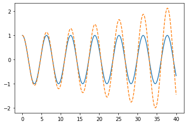
Let's try this with the same grid as before:
ts = np.linspace(0, 40, 1000 + 1)
y = rk2_ivp(f, [x_max, v_0], ts)
plt.plot(ts, np.cos(ts))
plt.plot(ts, y[:, 0], "--")
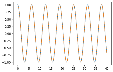
And, on a coarser grid:
ts = np.linspace(0, 40, 100 + 1)
y = rk2_ivp(f, [x_max, v_0], ts)
plt.plot(ts, np.cos(ts))
plt.plot(ts, y[:, 0], "--")

We can get the RK4 algorithm by keeping another non-zero term in the Taylor series:
$$ \mathbf{y}_{n+1} \approx \mathbf{y}_{n} + \frac{1}{6} (\mathbf{k}_1 + 2 \mathbf{k}_2 + 2 \mathbf{k}_3 + \mathbf{k}_4 ) \tag{2.0} $$$$ \mathbf{k}_1 = h \mathbf{f}(t_n,\, \mathbf{y}_n) \tag{2.1} $$$$ \mathbf{k}_2 = h \mathbf{f}(t_n + \frac{h}{2},\, \mathbf{y}_n + \frac{\mathrm{k}_1}{2}) \tag{2.2} $$$$ \mathbf{k}_3 = h \mathbf{f}(t_n + \frac{h}{2},\, \mathbf{y}_n + \frac{\mathrm{k}_2}{2}) \tag{2.3} $$$$ \mathbf{k}_4 = h \mathbf{f}(t_n + h,\, \mathbf{y}_n + \mathrm{k}_3) \tag{2.4} $$def rk4_ivp(f, init_y, t):
steps = len(t)
order = len(init_y)
y = np.empty((steps, order))
y[0] = init_y
for n in range(steps - 1):
h = t[n + 1] - t[n]
k1 = h * f(t[n], y[n]) # 2.1
k2 = h * f(t[n] + h / 2, y[n] + k1 / 2) # 2.2
k3 = h * f(t[n] + h / 2, y[n] + k2 / 2) # 2.3
k4 = h * f(t[n] + h, y[n] + k3) # 2.4
y[n + 1] = y[n] + 1 / 6 * (k1 + 2 * k2 + 2 * k3 + k4) # 2.0
return y
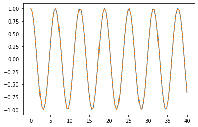
Let's try this with the same grid as before:
ts = np.linspace(0, 40, 100 + 1)
y = rk4_ivp(f, [x_max, v_0], ts)
plt.plot(ts, np.cos(ts))
plt.plot(ts, y[:, 0], "--")
%%timeit
ts = np.linspace(0, 40, 1000 + 1)
y = rk4_ivp(f, [x_max, v_0], ts)
Let's JIT both of these functions, and see if we can get a speedup!
import numba

f_jit = numba.njit(f)
rk4_ivp_jit = numba.njit(rk4_ivp)
%%timeit
ts = np.linspace(0, 40, 1000 + 1)
y = rk4_ivp_jit(f_jit, [x_max, v_0], ts)
How's that for almost 0 effort!
def rk45_ivp(f, init_y, t_range, tol=1e-8, attempt_steps=20):
    order = len(init_y)  # Number of equations

    y = [np.array(init_y)]
    t = [t_range[0]]
    err_sum = 0

    # Step size and limits to step size
    h = (t_range[1] - t_range[0]) / attempt_steps
    hmin = h / 64
    hmax = h * 64

    while t[-1] < t_range[1]:

        # Last step should just be exactly what is needed to finish
        if t[-1] + h > t_range[1]:
            h = t_range[1] - t[-1]

        # Compute k1 - k6 for evaluation and error estimate
        k1 = h * f(t[-1], y[-1])
        k2 = h * f(t[-1] + h / 4, y[-1] + k1 / 4)
        k3 = h * f(t[-1] + 3 * h / 8, y[-1] + 3 * k1 / 32 + 9 * k2 / 32)
        k4 = h * f(
            t[-1] + 12 * h / 13,
            y[-1] + 1932 * k1 / 2197 - 7200 * k2 / 2197 + 7296 * k3 / 2197,
        )
        k5 = h * f(
            t[-1] + h,
            y[-1] + 439 * k1 / 216 - 8 * k2 + 3680 * k3 / 513 - 845 * k4 / 4104,
        )
        k6 = h * f(
            t[-1] + h / 2,
            y[-1]
            + 8 * k1 / 27
            + 2 * k2
            - 3544 * k3 / 2565
            + 1859 * k4 / 4104
            - 11 * k5 / 40,
        )

        # Compute error from higher order RK calculation
        err = np.abs(
            k1 / 360 - 128 * k3 / 4275 - 2197 * k4 / 75240 + k5 / 50 + 2 * k6 / 55
        )

        # Compute factor to see if step size should be changed
        s = 0 if err[0] == 0 or err[1] == 0 else 0.84 * (tol * h / err[0]) ** 0.25

        lower_step = s < 0.75 and h > 2 * hmin
        raise_step = s > 1.5 and 2 * h < hmax
        no_change = not raise_step and not lower_step

        # Accept step and move on
        if err[0] < tol or err[1] < tol or no_change:
            y.append(
                y[-1] + 25 * k1 / 216 + 1408 * k3 / 2565 + 2197 * k4 / 4104 - k5 / 5
            )
            t.append(t[-1] + h)

        # Grow or shrink the step size if needed
        if lower_step:
            h /= 2
        elif raise_step:
            h *= 2

    return np.array(t), np.array(y)
ts = np.linspace(0, 40, 1000 + 1)
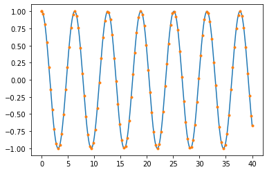
t, y = rk45_ivp(f, [x_max, v_0], [0, 40], 0.005)
plt.plot(ts, np.cos(ts))
plt.plot(t, y[:, 0], ".")

Let's compare it with the scipy algorithm:
import scipy.integrate
r45 = scipy.integrate.solve_ivp(f, [0, 40], [x_max, v_0], rtol=0.00001)
r45
plt.plot(ts, np.cos(ts))
plt.plot(r45.t, r45.y[0], ".")