Review

Week 13 Day 1: Review

Week	Monday	Wednesday	Friday
1	8-27 Introduction	8-29 Using Python part 1	8-31 Using Python part 2
2	9-03 Labor day	9-05 OO programming (4)	9-07 Error accumulation (2)
3	9-10 Numerical tools	9-12 Plotting (3)	9-14 Using git
4	9-17 Random numbers (5)	9-19 Monte Carlo (5)	9-21 Project selection
5	9-24 Integration rules (6)	9-26 MC Integration (6)	9-28 Numerical differentiation (7)
6	10-01 Vectorization (8)	10-03 Linear algebra (8)	10-05 Linear regression (8)
7	10-08 Structured tabular data	10-10 Cuts and histograms	10-12 Fall reading days
8	10-15 Generating distributions	10-17 Minimization and fitting	10-19 Fitting tools
9	10-22 Confidence intervals	10-24 Markov Chain Monte Carlo	10-26 Performance computing (14)
10	10-29 Intro to ODEs (9)	10-31 Runge–Kutta algorithm (9)	11-02 Solving ODE problems (9)
11	11-05 Fourier Series (10)	11-07 Fast Fourier Transform (10)	11-09 Project progress report
12	11-12 Veterans day	11-14 Project progress report	11-16 Filtering signals (10)
13	11-19 Review	11-21 Student requested topics	11-23 Thanksgiving
14	11-26 Static computation graphs	11-28 Applied ML topics	11-30 Sharing and documenting code
15	12-03 Term project presentations	12-05 Term project presentations	12-07 Term project presentations

import math
import numpy as np
import numba
import pandas as pd
import matplotlib.pyplot as plt
import seaborn as sns
from scipy import integrate, optimize, stats, misc

2.3: Error accumulation

Compare several summing methods to the very accurate "fsum"; which fairs best?

np.random.seed(42)
vals = np.random.normal(0, 1, 1_000_000)

fsummed = math.fsum(vals)

3.3: Using git

Describe the following commands:

git add -u .
git commit -m "hello"
git push
git grep "hello"

4.1: Integration rules

Integrate the following function. You should use tools provided; don't write your own integrator unless it is necessary for some reason!

$$ f(x) = \int _0 ^1 \sin(\cos x) \, dx \approx 0.73864... $$

(From Wolfram Alpha+from+x%3D0+to+1&lk=3))

def f(x):
    return np.sin(np.cos(x))

4.2: MC Integration

What situations would you want to use MC integration instead of a regular grid and an integration rule?

Integrate the above function with MC. Note there is not a built in function to do so, since it's so easy to do.

4.3: Numerical differentiation

Can you find a numerical derivative for the function above at 1/2? Analytic solution shown.

real_deriv = -np.cos(np.cos(0.5)) * np.sin(0.5)
real_deriv

-0.30635890918999453

5.3, 8.2, 8.3 : Fitting

We've already done a bit of this, so let's just hit a highlight or two.

Functions:

Interpolation: connect the dots. Cubic splines were probably the nicest visual interpolation method.
Linear regression: np.polyfit or np.linalg.lstsq
Non-linear least squares: optimize.curve_fit

Distributions:

Binned fits: See above, be careful and include error
Unbinned fits: NLL (use optimize.minimize or custom package)

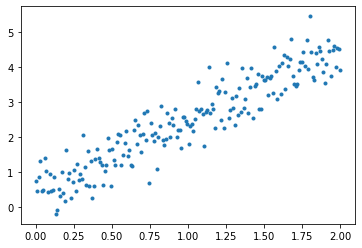
Try a quick polyfit here:

np.random.seed(42)
x = np.linspace(0, 2, 200)
y = x * 2 + 0.5 + np.random.normal(0, 0.5, 200)

# Add fit here

plt.plot(x, y, ".")

[<matplotlib.lines.Line2D at 0x7f05e8bf85d0>]

6.1, 6.2: Structured tabular data and cuts

Play with the following dataframe. Make a scatter plot of sepal_width vs. sepal_length with each of the three species a different color.

df = pd.read_csv(
    "https://raw.githubusercontent.com/mwaskom/seaborn-data/master/iris.csv"
)

df.head()

	sepal_length	sepal_width	petal_length	petal_width	species
0	5.1	3.5	1.4	0.2	setosa
1	4.9	3.0	1.4	0.2	setosa
2	4.7	3.2	1.3	0.2	setosa
3	4.6	3.1	1.5	0.2	setosa
4	5.0	3.6	1.4	0.2	setosa

Note, we could do this with seaborn:

sns.scatterplot("sepal_length", "sepal_width", "species", data=df)

<matplotlib.axes._subplots.AxesSubplot at 0x7f05e84938d0>

9.2: MCMC

Let's look at the metropolis algorithm (MCMC but without computing a posterior, so simpler) to produce samples from $\sin(x)**2 / x**2$

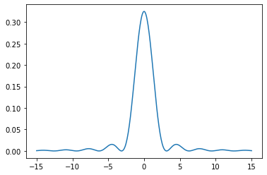
def p(x):
    return np.sin(x) ** 2 / x ** 2

Normalization not needed for algorithm, but makes the plots line up:

integ, err = integrate.quad(p, -15, 15.000001)
print(integ, err)

3.07712984526598 1.2636296904677824e-09

x1 = np.linspace(-15, 15, 400)
y1 = p(x1) / integ

Now compute the metropolis algorithm:

samples = 100_000
sigma = 10
x = np.empty(samples + 1)
x[0] = np.random.rand()

for i in range(samples):
    # suggest new position xStar
    ...

    # Compute alpha - the fractional chance of moving to a new point
    ...

    # Accept/reject based on alpha
    ...

    # Add the current (moved?) point
    ...

plt.plot(x1, y1)
# plt.hist(x[500:], density=True, bins=100)
# plt.yscale('log')
plt.show()

Side project: This is great, but very slow. We can make this a function, and add a couple of @numba.njit's, and get a massive speedup!

10.2: Runge-Kutta algorithms

Let's look at ODEs, and revisit the RK2 algorithm. Remember you can do the following:

$$ \mathbf{u} = \left( \begin{matrix} \dot{x} \\ x \end{matrix} \right) $$$$ \mathbf{f}(t, \mathbf{u}) = \dot{\mathbf{u}} $$

To get a first order ODE.

We'll start with one, though:

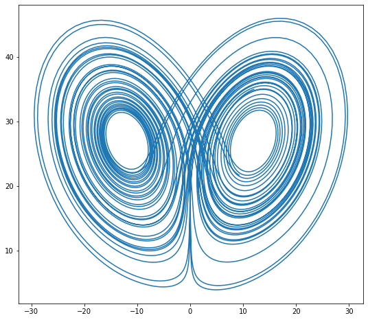
$$ u = \left( \begin{matrix} x \\ y \\ z \end{matrix} \right) $$$$ \dot{u} = \left( \begin{matrix} \sigma (y - x) \\ \rho x - x z - y \\ x y - \beta z \end{matrix} \right) $$

Constants given below. (example from Bokeh)

sigma = 10
rho = 28
beta = 8 / 3
theta = 3 * np.pi / 4


def lorenz(t, xyz):
    x, y, z = xyz
    x_dot = sigma * (y - x)
    y_dot = x * rho - x * z - y
    z_dot = x * y - beta * z
    return np.array([x_dot, y_dot, z_dot])

initial = (-10, -7, 35)
t = np.arange(0, 50, 0.006)

RK2

def rk2_ivp(f, init_y, t):
    steps = len(t)
    order = len(init_y)

    y = np.empty((steps, order))
    y[0] = init_y

    for n in range(steps - 1):
        h = t[n + 1] - t[n]

        k1 = h * f(t[n], y[n])  # 1.1
        k2 = h * f(t[n] + h / 2, y[n] + k1 / 2)  # 1.2

        y[n + 1] = y[n] + k2  # 1.0

    return y

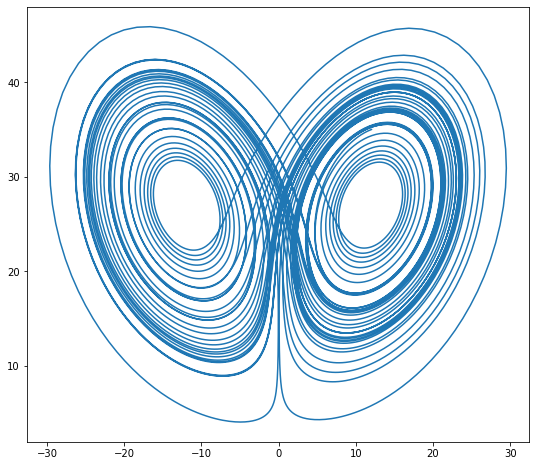
xyz = rk2_ivp(lorenz, initial, t)
xprime = np.cos(theta) * xyz[:, 0] - np.sin(theta) * xyz[:, 1]

plt.figure(figsize=(9, 8))
plt.plot(xprime, xyz[:, 2])
plt.show()

RK4

def rk4_ivp(f, init_y, t):
    steps = len(t)
    order = len(init_y)

    y = np.empty((steps, order))
    y[0] = init_y

    for n in range(steps - 1):
        h = t[n + 1] - t[n]

        k1 = h * f(t[n], y[n])  # 2.1
        k2 = h * f(t[n] + h / 2, y[n] + k1 / 2)  # 2.2
        k3 = h * f(t[n] + h / 2, y[n] + k2 / 2)  # 2.3
        k4 = h * f(t[n] + h, y[n] + k3)  # 2.4

        y[n + 1] = y[n] + 1 / 6 * (k1 + 2 * k2 + 2 * k3 + k4)  # 2.0

    return y

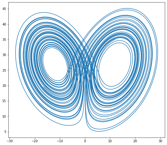
xyz = rk4_ivp(lorenz, initial, t)
xprime = np.cos(theta) * xyz[:, 0] - np.sin(theta) * xyz[:, 1]

plt.figure(figsize=(9, 8))
plt.plot(xprime, xyz[:, 2])
plt.show()

Solve IVP

res = integrate.solve_ivp(lorenz, (0, 100), initial, t_eval=t)
xprime = np.cos(theta) * res.y[0] - np.sin(theta) * res.y[1]

plt.figure(figsize=(9, 8))
plt.plot(xprime, res.y[2])
plt.show()

Ode Int

Let's try this with ODE Int, since that's in older SciPy's. The main difference is the reversed order for f, and

def lorenz_flip(xyz, t):
    return lorenz(t, xyz)


xyz = integrate.odeint(lorenz_flip, initial, t)
xprime = np.cos(theta) * xyz[:, 0] - np.sin(theta) * xyz[:, 1]

plt.figure(figsize=(9, 8))
plt.plot(xprime, xyz[:, 2])
plt.show()