import seaborn as sns
import pandas as pd
import numpy as np
import matplotlib.pyplot as plt
Let's start with the following table of data:
state = np.random.RandomState(42)
time = np.linspace(0, 2, 10)
xs = time * 0.3 + (state.rand(10) - 0.5) * 0.1
ys = -(time ** 2) + 2 * time + (state.rand(10) - 0.5) * 0.1
print("      time          x          y\n")
for t, x, y in zip(time, xs, ys):
    print(f"{t:10.4} {x:10.4} {y:10.4}")
We would like to view and work with this as a coherent single entity. If we chose to use a matrix, we'd have some issues:
- Our axes are inherently different - operations along columns make sense, rows... Not so much.
- One of the axis has labels (time, x, and y) that we'd lose, making our code harder to read
- What happens if we have different data types?
- Normal matrix operations (like multiplication) don't really make sense
Let's just look at what a Pandas DataFrame would look like, then we'll talk a bit more about them. Note that there are a ton of ways to make a DataFrame. And we have some choices we will ignore for now.
df = pd.DataFrame({"time": time, "x": xs, "y": ys})
df
Our time would make a better index than the default 0,1,2,...,9, so let's try that:
df.set_index("time", inplace=True)
df
# df.index = pd.to_timedelta(df.index, unit='s')
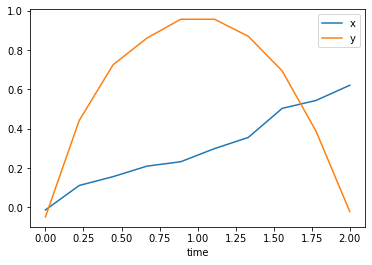
df.plot()
# df.plot('x', 'y', kind='scatter');
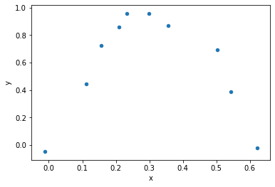
df.plot.scatter("x", "y")
There are two ways to access columns:
df["x"]
df.x
A column is a "Series": That's like a 1D array but with an index and possibly a name attached. The Series align on index instead of location - if you add two Series, matching indexed value will add.
The ['x'] syntax is more general, but the .x syntax is shorter, and much nicer in a notebook. It doesn't work for setting brand new columns, or if the name of a column is not valid in Python or would overwrite an existing property or method.
DataFrames and Series follow the array protocol, so numpy operation work on them too:
df["r"] = np.sqrt(df.x ** 2 + df.y ** 2)
df
DataFrames are designed to make it easy to add and operate on columns; you should not in general be adding new rows (this should tell you what the internal memory layout must be like).
Note that you can use .apply to apply a function to a DataFrame with a bit more control, or .applymap to apply a function element-wise to a DataFrame or Series (but the function is a Python function, so the loop must happen in Python so it is slower than .apply)
Pandas features
Pandas design:
- Make everything as Pythonic as possible. Even if that means there are many ways of doing things.
- Design around everyday usage rather than theory
Features:
- Index types: Several custom arrays with extra features for types of indexes
- Including hierarchical indexes, which allow multidimensional-like data to be used
- Series: A 1D array with an attached index
- New types: Powerful datetime and timedelta features, including special calender support, periodic times, etc.
- Categorical support (a bit more powerful than sets)
- DataFrame: a table of data with indexes and headers
- Great input/output support for lots of data formats (
.csv, Excel, many more) - Great output display, notebook support
- Amazing data manipulation
- Like Numpy, can be a standard for other statistical packages
Constructing and writing a dataframe
- See the DataFrame's help for a massive list of options.
- Reading in a DataFrame is done with the
pd.read_*functions. - Writing a DataFrame is done with the
df.to_*methods.
See Table 5-1: Possible data inputs to DataFrame constructor in Python for Data Analysis, 2nd edition, by Wes McKinney. Also Chapter 6 for reading/writing DataFrames.
Indexing
df[x] is a special case - it behaves differently depending on the arguments - columns normally but some cases are rows (such as when using a boolean Series). When doing something specific, use the specialized accessors:
df[column]: Select a columndf.loc[row, column]: Indexing by namesdf.iloc[row, column]: Indexing by numberatandiatare available for single values.
Note that using a list is different than a tuple in an indexing expression in Pandas.
See Table 5.4 for ways to index a DataFrame
Indexing options with DataFrame in Python for Data Analysis, 2nd edition, by Wes McKinney.
df = sns.load_dataset("iris")
df
A few things of note:
- No column makes sense as an index here - we'll just leave the numerical index.
- We have a categorical column - but it didn't read in as a categorical datatype! That's easy to fix:
df.species = df.species.astype("category")
We can quickly get some information about the data:
df.describe()
df.info()
df.dtypes
Accessors
You can use an "accessor" (Pandas terminology) to perform operations on series as a specific type:
.str: string methods that act on the series.cat: Operations on categories.dt: Datetime operations.plot: Serves two purposes, either acts like a plot function or gives you access to other types of plots
df.species.str.capitalize().head()
df.species.cat.categories
We can use a boolean Series to select rows from a DataFrame (or another Series):
df[df.species == "setosa"].head()
Let's select just two rows of our table: (Note: this must be a list, not a tuple)
df[["sepal_length", "sepal_width"]].head()
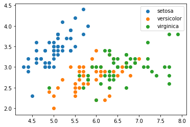
We can combine what we've learned:
(notice the automatic x and y axis labels)
fig, ax = plt.subplots()
for i, category in enumerate(df.species.cat.categories):
    df[df.species == category].plot.scatter(
        "sepal_length", "sepal_width", label=category, c=f"C{i}", ax=ax
    )
plt.show()
MatPlotLib now has better support for Pandas, which makes this a bit easier:
fig, ax = plt.subplots()
for category in df.species.cat.categories:
    ax.scatter(
        "sepal_length", "sepal_width", data=df[df.species == category], label=category
    )
plt.legend()
plt.show()
We could make this even nicer with a groupby, which returns a group you can iterate over to get the name and dataframe:
fig, ax = plt.subplots()
for name, group in df.groupby("species"):
    ax.scatter("sepal_length", "sepal_width", data=group, label=name)
plt.legend()
plt.show()
Pandas supports lots more, like database style merges and joins, etc.
In general, the best thing to do with Pandas is search and look around to see if the functionality you want is there. Avoid loops and anything that looks ugly until you are sure it's the only what to do what you want.
Pandas can be seen as similar to:
- Excel
- R
- SQL
- SAS
- Stata
- ROOT (some parts)
Learn more at:
- Pandas website
- Our recommended book (available on the UC libraries online)
- 10 minutes to Pandas


