Fitting Tools

Week 8 Day 3: Fitting tools

Objectives:

Look again at fitting tools
Set up a project in git (review of git, project structure)

Note about crash last time!

GooFit and LmFit both seem to have compiled code that expects OpenMP - and at least on my Mac, they were linked with different OpenMP libraries (Anaconda's Intel libomp for LmFit, and HomeBrew's libomp for GooFit). So that's why it crashed. I've reinstalled GooFit without OpenMP for now.

GooFit

If you really want to try GooFit, you can try this on OSC:

!pip install --user scikit-build cmake
!PATH=$HOME/.local/bin:$PATH pip install --user --verbose goofit

The extra requirements here are partially to ensure it gets the highest level of optimization, and partially requirements that will eventually go away.

If you are on macOS, scikit-build is broken, you'll need !pip install scikit-build==0.6.1.

from scipy.stats import norm, multivariate_normal
import matplotlib.pyplot as plt
import numpy as np

Prepare data

We'll be making a set of data out of a Gaussian + linear.

state = np.random.RandomState(42)
gauss_part = state.normal(1, 2, size=100_000)
lin_part = state.uniform(low=-10, high=10, size=50_000)
total_rand = np.concatenate([gauss_part, lin_part])

import goofit

We need an observable, with a range from -10 to 10.

x = goofit.Observable("x", -10, 10)

We can make an unbinned (or binned) dataset; we need to list the variables it will contain.

data = goofit.UnbinnedDataSet(x)

Let's read in data. GooFit will default to throwing an error if you input a value that is outside the range (-10 to 10 in this case), but we can pass filter=True to simply ignore those values instead.

data.from_matrix([total_rand], filter=True)

If you display a PDF in the notebook, you get a nice pretty-printed version of it's documentation:

goofit.PolynomialPdf

If the Gaussian is the potato, what is the polynomial? Bread? Milk? Nothing exotic, at any rate. The GooFit version does have some subtleties, to allow for polynomials over an arbitrary number¹ of dimensions:

$$ P(\vec x; \vec a, \vec x_0, N) = \sum\limits_{p_1+p_2+\ldots+p_n \le N} a_{p_1p_2\ldots p_n} \prod\limits_{i=1}^n (\vec x - \vec x_0)_i^{p_i} $$

where $N$ is the highest degree of the polynomial and $n$ is the number of dimensions. The constructor takes a vector of observables, denoted $\vec x$ above; a vector of coefficients, $\vec a$, a vector of optional offsets $\vec x_0$ (if not specified, these default to zero), and the maximum degree $N$. The coefficients are in the order $a_{p_0p_0\ldots p_0}, a_{p_1p_0\ldots p_0}, \ldots a_{p_Np_0\ldots p_0}, a_{p_0p_1\ldots p_0}, a_{p_1p_1\ldots p_0}, \ldots a_{p_0p_0\ldots p_N}$. In other words, start at the index for the constant term, and increment the power of the leftmost observable. Every time the sum of the powers reaches $N$, reset the leftmost power to zero and increment the next-leftmost. When the next-leftmost reaches $N$, reset it to zero and increment the third-leftmost, and so on.

An example may be helpful; for two dimensions $x$ and $y$, and a maximum power of 3, the order is $a_{00}, a_{10}, a_{20}, a_{30}, a_{01}, a_{11}, a_{21}, a_{02}, a_{12}, a_{03}$. This can be visualised as picking boxes out of a matrix and discarding the ones where the powers exceed the maximum:

$$ \begin{array}{cccc} 9: x^0y^3 & - & - & - \\ 7: x^0y^2 & 8: x^1y^2 & - & - \\ 4: x^0y^1 & 5: x^1y^1 & 6: x^2y^1 & - \\ 0: x^0y^0 & 1: x^1y^0 & 2: x^2y^0 & 3: x^3y^0 \\ \end{array} $$

starting in the lower-lefthand corner and going right, then up.

There is also a simpler version of the constructor for the case of a polynomial with only one dimension; it takes the observable, a vector of coefficients, an optional offset, and the lowest (not highest) degree of the polynomial; the latter two both default to zero. In this case the order of the coefficients is from lowest to highest power.

sufficed.

Although being honest, just supporting the special cases of one and two would likely have↩

The fitting variables and PDFs need to be setup next.

a = goofit.Variable("a", 0, 0, 1)
linear = goofit.PolynomialPdf("linear", x, [a])

mu = goofit.Variable("mu", 0, -10, 10)
sigma = goofit.Variable("sigma", 1, 0, 5)
gauss = goofit.GaussianPdf("gauss", x, mu, sigma)

We can add multiple PDFs with fractions for each

frac = goofit.Variable("frac", 0.5, 0, 1)
total = goofit.AddPdf("tot", [frac], [gauss, linear])

And, we can fit a PDF to data:

minimum = total.fitTo(data)

MnSeedGenerator: for initial parameters FCN = 841645.2784155
MnSeedGenerator: Initial state:   - FCN =   841645.2784155 Edm =        54488 NCalls =     19
MnSeedGenerator: Negative G2 found - new state:   - FCN =   841645.2784155 Edm =      54480.8 NCalls =     28
VariableMetric: start iterating until Edm is < 0.0001
VariableMetric: Initial state   - FCN =   841645.2784155 Edm =      54480.8 NCalls =     28
VariableMetric: Iteration #   0 - FCN =   841645.2784155 Edm =      54480.8 NCalls =     28
VariableMetric: Iteration #   1 - FCN =   805725.7295866 Edm =      5523.23 NCalls =     39
VariableMetric: Iteration #   2 - FCN =    795403.425499 Edm =      1918.81 NCalls =     50
VariableMetric: Iteration #   3 - FCN =   792737.6548792 Edm =      3.47229 NCalls =     60
VariableMetric: Iteration #   4 - FCN =   792732.0268167 Edm =    0.0484444 NCalls =     70
VariableMetric: Iteration #   5 - FCN =   792731.9534002 Edm =   0.00389431 NCalls =     80
VariableMetric: Iteration #   6 - FCN =   792731.9490078 Edm =  2.48375e-07 NCalls =     90

Minuit did successfully converge.
# of function calls: 90
minimum function Value: 792731.9490078
minimum edm: 2.483749293692e-07
minimum internal state vector: LAVector parameters:
     0.3420860135755
     0.1005454536517
    -0.1996606468995
     -1.068843201795

minimum internal covariance matrix: LASymMatrix parameters:
  2.0181161e-05  2.2787992e-08  6.9267333e-06              0
  2.2787992e-08  6.3784342e-07  2.0316983e-08              0
  6.9267333e-06  2.0316983e-08  9.7223226e-06              0
              0              0              0              2


# ext. ||   Name    ||   type  ||     Value     ||  Error +/- 

   0   ||      frac || limited ||     0.6677264820844 ||0.001496251179233
   1   ||        mu || limited ||      1.003761304242 ||0.005618793663826
   2   ||     sigma || limited ||      2.004158173175 ||0.005402504047424
   3   ||         a || limited ||    0.06167774468737 ||0.2024321074636




The minimization took: 945.73 ms
Average time per call: 10.511 ms

The variables are changed in place (mutated):

print(frac)

frac: 0.6677 +/- 0.0015 [0, 1] Fitter index: 0

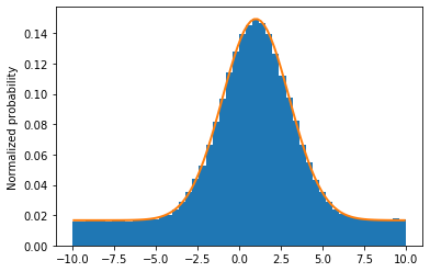
Let's look at a plot.

grid, pts = total.evaluatePdf(x)
xvals = grid.to_numpy().flatten()

fig, ax = plt.subplots(figsize=(6, 4))
ax.hist(total_rand, bins=50, range=(-10, 10), density=True)
ax.plot(xvals, pts, linewidth=2)
# ax.set_xlabel('xvar')
ax.set_ylabel("Normalized probability")
ax.set_ylim(ymin=0)
plt.show()