import numpy as np
import scipy.integrate
import matplotlib.pyplot as plt
Let's look now at ODEs. Let's take one of the most famous physics examples:
$$ F_k(x) = m \ddot{x} = - k x $$This is the equation for the restoring force of a spring - this is an analytically solvable equation with the solution:
$$ x(t) = x_\mathrm{max} \cos\left(\sqrt{\frac{k}{m}} t\right) $$This is harmonic motion. Notice that we had to set some initial conditions here; the value of $x(0)=x_{\max}$ and $\dot{x}(0)=0$.
Now let's try to solve this numerically. We'll learn much better ways to do this, but for now, we are just going to use time steps and Euler’s algorithm.
Note: I learned something today from the IPython release notes. Type
\Deltathen press tab. Perfect for Python 3!
</font>
ΔT = 0.01  # timestep
steps = 1_000  # Total number of steps
x_max = 1  # Size of x max
v_0 = 0
koverm = 1  # k / m

# Compute the final values of t for plotting
ts = np.linspace(0, ΔT * (steps - 1), steps)
xs = np.empty(steps)
vs = np.empty(steps)

xs[0] = x_max
vs[0] = v_0

for i in range(steps - 1):
    # Compute a based on *current* position
    a = -koverm * xs[i]

    # Compute next velocity
    vs[i + 1] = vs[i] - a * ΔT

    # Compute next position
    xs[i + 1] = xs[i] - vs[i] * ΔT
plt.plot(ts, xs)

For a better solver, we need to rewrite the equation to a standard form, a vector of first order ODEs:
$$ \ddot{x} = - \frac{k}{m} x $$As a series of first order equations by writing
$$ u = \left( \begin{matrix} \dot{x} \\ x \end{matrix} \right) $$Then,
$$ \dot{u} = \left( \begin{matrix} \ddot{x} \\ \dot{x} \end{matrix} \right) = \left( \begin{matrix} - \frac{k}{m} x \\ \dot{x} \end{matrix} \right) $$def f(t, y):
"Y has two elements, x and v"
return -koverm * y[1], y[0]
res = scipy.integrate.solve_ivp(f, [ts[0], ts[-1]], [1, 0], t_eval=ts)
print(res.message)
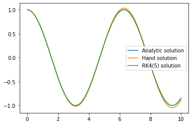
plt.plot(ts, np.cos(ts), label="Analytic solution")
plt.plot(ts, xs, label="Hand solution")
plt.plot(res.t, res.y[0], label="RK4(5) solution")
plt.legend()
plt.show()