Errors
- The most serious sort of error: A segfault
- Issue with the underlying compiled code
- Very rare in Python itself, can be intentionally caused or a bug in libraries
- Most errors are "Exceptions": A control flow feature in Python - and you can act on and work with them!
- You can even use Exceptions for things that are not errors
Exceptions
Exceptions are designed to interrupt the control flow for "exceptional" events. This makes writing safe code much easier - could you imagine if every function had to return an error status, and you had to check the status and also return your own error status if it was bad? (If you can imagine it, congratulations, you can write C code).
Imagine this:
def f(x):
    s = 0
    for i in range(10):
        if x == 0:
            return 0, "Error in calculations"
        s += i / x
    return s, ""


value, error = f(0)

if error:
    print(error)
else:
    print(value)
Compare to this:
def f(x):
    s = 0
    for i in range(10):
        if x == 0:
            raise RuntimeError("Error in calculations")
        s += i / x
    return s


try:
    value = f(0)
    print(value)
except RuntimeError as e:
    print(e)

# Try running this without the try/catch to see the full exception printout
The benefits to the second example:
- This nests; the in-between functions don't need to know about the Exception in the inner function or the check in the outer function
- Exceptions just bubble up through the stack
- This keeps errors from interfering with the function return values
- If we remove the Exception checking, we get a Python error message
- If we remove the check, Python automatically throws an exception when you divide by zero!
- The code is faster if we don't throw an exception often
def f(x):
    s = 0
    for i in range(10):
        s += i / x
    return s


try:
    value = f(0)
    print(value)
except ZeroDivisionError as e:
    print(e)
So now we see that Python has a ZeroDivisionError, and it is raised when you divide by zero. So we can now make a function that can take 0's without making an explicit check for 0!
def direction_xy(vec):
    """
    This takes a direction vector vec[0], vec[1], vec[2], and
    returns the x and y componets of a vector with length 1 z component.
    If the length of z is 0, returns [0,0].
    """

    try:
        return vec[0] / vec[2], vec[1] / vec[2]
    except ZeroDivisionError:
        return vec[0] * 0, vec[1] * 0


def direction_xy_classic(vec):
    if vec[2] == 0:
        return vec[0] * 0, vec[1] * 0
    else:
        return vec[0] / vec[2], vec[1] / vec[2]
The version that does not check will be faster when the exception is not caught - you are not paying for an extra check:
%%timeit
direction_xy((1, 2, 3))
%%timeit
direction_xy_classic((1, 2, 3))
However, the exception catching mechanism is slower than the normal control flow if it does get caught a lot:
%%timeit
direction_xy((1, 2, 0))
%%timeit
direction_xy_classic((1, 2, 0))
Exception throwing
You have a large collection of standard exceptions in Python:
You can make a new one trivially:
class MyException(RuntimeError):
    pass
Exception catching
You put the code that might throw an exception in a try: block.
You put the possible exception catching parts in one or more except Name: block following that. It contains the name of the exception type - you can list multiple exception type to catch, and any subclasses will also be caught. You can optionally keep a reference to the exception to use by using as. You can even reraise the exception with raise. You can also raise Err() from y (Python 3) to give users a more explicit traceback. Or raise Err() from None to give a less explicit traceback (hides the original exception).
You optionally can put in a else block which runs if no exceptions were caught, and a finally block, which runs no-matter-what (for cleanup, usually). See this or PEP 341.
Here's a playground for you. Try changing the caught exception type to RuntimeError and then another type of error, and experiment a bit.
class MyException(RuntimeError):
    pass


def f():
    raise MyException()


try:
    f()
except MyException:
    print("Caught Exception!")
try:
    import some_fancy_printout_package_that_does_not_exist
except ImportError:
    some_fancy_printout_package_that_does_not_exist = None

if some_fancy_printout_package_that_does_not_exist:
    print("Using fancy printout")
else:
    print("Not using fancy printout")
In Python, it is often better to ask for forgiveness than to ask for permission.
This is can be better in more ways than just performance. What happens if you check for the existence of a file, find it exists, then try to open it, just to find it was deleted in the meantime?
from scipy.stats import norm, multivariate_normal
import matplotlib.pyplot as plt
import numpy as np
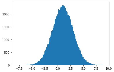
gauss_X = norm.rvs(1, 2, 100_000)
plt.hist(gauss_X, bins="auto")
plt.show()
mean, sigma = norm.fit(gauss_X)
print(f"mean = {mean}, sigma = {sigma}")
Note that we have no error information, no pretty much anything... Just a result.
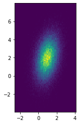
And, we can make a ND Gaussian, including covariance:
XY = multivariate_normal.rvs([1, 2], cov=[[0.5, 0.3], [0.3, 2]], size=100_000)
plt.hist2d(*XY.T, bins=100)
plt.gca().set_aspect("equal")
plt.show()
But... Multivariate norm is missing a fit function! Ugh...
from scipy.optimize import curve_fit, minimize
Reminder, curve fits wants a function that take 1 data parameter followed by functional parameters:
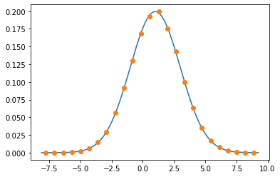
vals, edges = np.histogram(gauss_X, bins=25, density=True)
centers = (edges[1:] + edges[:-1]) / 2
curve_fit(norm.pdf, centers, vals, [1, 1])
xs = np.linspace(edges[0], edges[-1], 500)
plt.plot(xs, norm.pdf(xs, 1, 2))
plt.plot(centers, vals, "o")
plt.show()
Unbinned is not quite as easy, but we can still do it explicitly. We want to minimize an NLL:
$$ NLL = -\sum_i \ln\left( P(x_i) \right) $$The minimize function in scipy.optimize takes:
- A function to minimize. It must take an iterable of parameters as the first argument. You can pass through other arguments using
args. - An initial guess for parameters
- Optional args to pass through.
def NLL_gauss(params, x):
    mu, sigma = params
    y = norm.pdf(x, mu, sigma)
    return -np.sum(np.log(y))
minimize(NLL_gauss, [0.9, 1.8], args=(gauss_X,))
type(_)
Try methods to fix the success=False:
- Set a low
tol=parameter - Increase the number of samples
- Try
method = 'Nelder-Mead'
Warning: we've skipped something important by using the Gaussian pdf from Scipy: It is normalized! We need normalized PDF functions for this to work. If you write your own, you need a normalized function.
Other tools
So, this can be done by hand; but several things are missing:
- Easy ways to build distribution PDFs, especially combinations
- Even would be nicer if high-speed/GPU calculations possible
- Extra error information, including asymmetric errors
- Pretty fitting API
- Better parameter limit control, and nice API
- Automatic derivatives of fitting function (though you can pass a manual one!)
Some packages exist:
- LMFit: Seems to be one of the common tools outside of HEP - it doesn't seem to like unbinned fits, though.
- iMinuit and probfit: HEP tools made available to normal Pythonistas. Probfit pip package broken on Python 3.
- RooFit: A ROOT tool for fitting. Very powerful, very slow, very hard to install and keep from segfaulting
- GooFit: A GPU/OpenMP tool, fast but new PDFs must be added in C++/CUDA.
The general design is somewhat similar. You need the following pieces:
- Parameters: variables you minimize
- Data: The input data - often provides Observables for each dimension
- Models: Common "parts" that you can combine
- Normalization: When fitting, you need to normalize for the NLL to work. (Missing in LMFit?)
- Fitter: something to do the fitting
from lmfit.models import GaussianModel, LinearModel
gauss_part = np.random.normal(1, 2, size=100_000)
lin_part = np.random.uniform(low=-10, high=10, size=50_000)
total_rand = np.concatenate([gauss_part, lin_part])
model = GaussianModel(prefix="gauss_") + LinearModel(prefix="lin_")
vals, edges = np.histogram(total_rand, bins=25, density=True)
centers = (edges[1:] + edges[:-1]) / 2
res = model.fit(vals, x=centers)
print(res.success)
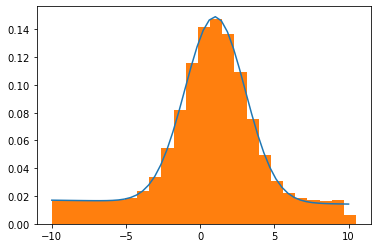
x = np.linspace(-10, 10)
y = model.eval(params=res.params, x=x)
plt.plot(x, y)
plt.hist(total_rand, bins=25, density=True)
plt.show()
GooFit
If you really want to try GooFit, you can try this on OSC:
!pip install --user scikit-build cmake
!PATH=$HOME/.local/bin:$PATH pip install --user --verbose goofit
The extra requirements here are partially to ensure it gets the highest level of optimization, and partially requirements that will eventually go away.
If you are on macOS, scikit-build is broken, you'll need !pip install scikit-build==0.6.1.
import goofit
x = goofit.Observable("x", -10, 10)
data = goofit.UnbinnedDataSet(x)
data.from_matrix([total_rand], filter=True)
goofit.PolynomialPdf
a = goofit.Variable("a", 0, 0, 1)
linear = goofit.PolynomialPdf("linear", x, [a])
mu = goofit.Variable("mu", 0, -10, 10)
sigma = goofit.Variable("sigma", 1, 0, 5)
gauss = goofit.GaussianPdf("gauss", x, mu, sigma)
frac = goofit.Variable("frac", 0.5, 0, 1)
total = goofit.AddPdf("tot", [frac], [gauss, linear])
minimum = total.fitTo(data)
print(frac)
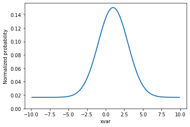
Let's look at a plot.
grid, pts = total.evaluatePdf(x)
total.setData(grid)

fig, ax = plt.subplots(figsize=(6, 4))
v = ax.plot(grid.to_numpy().flatten(), pts, linewidth=2)[0]
ax.set_xlabel("xvar")
ax.set_ylabel("Normalized probability")
ax.set_ylim(ymin=0)
plt.show()

