Debugging
Using a debugger has several parts:
- Starting the debugger
- Classic way:
import pdb; pdb.set_trace()(This is the standard library debugger) - Python 3.7 way:
breakpoint()(This will start the current debugger) - IPython offers
%debugto jump in after an error is raised! (likepdb.pm()) - You can also start at the beginning (see docs)
- Classic way:
- Controlling the debugger
pyb(andipydb) are sort of based on classic debugging tools - the syntax is a bit odd, but will be useful in other languages.- A common term is the "stack", short in this case for the "call-stack", the series of functions that call each other to get to the current point.
- Note that the "stack" is also a term for memory locations in compiled programs - and is unrelated to this usage.
| short | name | action | Names in other debuggers |
|---|---|---|---|
h |
help |
Print out help | |
p |
print |
Print out the value of a variable or expression | |
u |
up |
Go up one in the stack | |
d |
down |
Go down one in the stack | |
w |
where |
Show you where you are | Stack trace |
s |
step |
Move forward one computation | Step in |
n |
next |
More forward one line | Step over |
c |
continue |
Continue on till next stop | |
b |
breakpoint |
Set a breakpoint somehere | |
q |
quit |
Quit |
## A program to debug
def simple_function(div):
    simple_x = 2
    simple_y = div

    # import pdb; pdb.set_trace()

    return fancy_function(simple_x, simple_y)


def fancy_function(x, y):
    r = x / y
    return r
# simple_function(0)
# %debug
# simple_function(2)
# import pdb
# pdb.run('simple_function(0)')
Other tools: Tracing
Some IDEs, like PyCharm, may offer enhanced and partially graphical debuggers. And, in Python 3.7, the new built-in breakpoint() can call the fancy debugger instead of the builtin one!
Let's look at something similar: Tracing. If you have a complex piece of Python code and you want to have an idea of what the control flow looks like, you can trace it.
%%writefile simple.py

## A program to debug
def simple_function(div):
    simple_x = 2
    simple_y = div

    return fancy_function(simple_x, simple_y)


def fancy_function(x, y):
    r = x / y
    return r


def main():
    print(simple_function(2))


if __name__ == "__main__":
    main()
!python simple.py
!python -m trace --trace simple.py
!python -m trace --listfuncs simple.py
import numpy as np
import matplotlib.pyplot as plt
import scipy.integrate
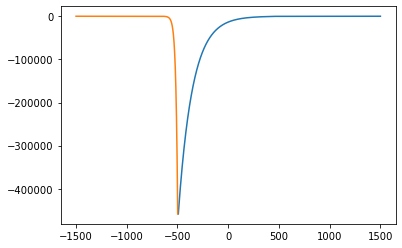
Again, we write this as a set of first order equations:
$$ u = \left(\begin{matrix}\psi' \\ \psi\end{matrix}\right) $$$$ u' = \left(\begin{matrix}\psi'' \\ \psi'\end{matrix}\right) = \left(\begin{matrix}\left( \frac{2 m}{\hbar^2} V_0 - \kappa^2 \right) \psi \\ \psi'\end{matrix}\right) $$where we set $V_0$ to $0$ when $|x|$ is larger than $a$. Boundary conditions:
$$ \psi(x_\mathrm{max}) = e^{-\kappa x_\mathrm{max}} \\ \psi(-x_\mathrm{max}) = e^{-\kappa x_\mathrm{max}} $$Double click to see broken code for solve_bvp (in a live notebook, not a viewer).
""" From "COMPUTATIONAL PHYSICS" & "COMPUTER PROBLEMS in PHYSICS"
by RH Landau, MJ Paez, and CC Bordeianu (deceased)
Copyright R Landau, Oregon State Unv, MJ Paez, Univ Antioquia,
C Bordeianu, Univ Bucharest, 2017.
Please respect copyright & acknowledge our work."""
# QuantumEigen.py: Finds E and psi via rk4 + bisection
# mass/((hbar*c)**2)= 940MeV/(197.33MeV-fm)**2 =0.4829
# well width=20.0 fm, depth 10 MeV, Wave function not normalized.
import numpy as np
import matplotlib.pyplot as plt
eps = 1e-3 # Precision
n_steps = 501
E = -17 # E guess
h = 0.04
count_max = 100
Emax = 1.1 * E # E limits
Emin = E / 1.1
def f(x, y, E):
return np.array([y[1], -0.4829 * (E - V(x)) * y[0]])
def V(x):
# Well depth
return -16 if abs(x) < 10 else 0
def rk4(t, y, h, Neqs, E):
ydumb = np.zeros((Neqs), float)
k1 = np.zeros((Neqs), float)
k2 = np.zeros((Neqs), float)
k3 = np.zeros((Neqs), float)
k4 = np.zeros((Neqs), float)
F = f(t, y, E)
k1 = h * F
ydumb = y + k1 / 2
F = f(t + h / 2, ydumb, E)
k2 = h * F
ydumb = y + k2 / 2
F = f(t + h / 2, ydumb, E)
k3 = h * F
ydumb = y + k3
F = f(t + h, ydumb, E)
k4 = h * F
y += (k1 + 2 * (k2 + k3) + k4) / 6
def diff(E, h):
i_match = n_steps // 3 # Matching radius
nL = i_match + 1
y = np.array([1e-15, 1e-15 * np.sqrt(-E * 0.4829)]) # Initial left wf
for ix in range(0, nL + 1):
x = h * (ix - n_steps / 2)
rk4(x, y, h, 2, E)
left = y[1] / y[0] # Log derivative
y[0] = 1e-15
# For even; reverse for odd
y[1] = -y[0] * np.sqrt(-E * 0.4829) # Initialize R wf
for ix in range(n_steps, nL + 1, -1):
x = h * (ix + 1 - n_steps / 2)
rk4(x, y, -h, 2, E)
right = y[1] / y[0] # Log derivative
return (left - right) / (left + right)
def plot(E, h):
# Repeat integrations for plot
x = 0.0
n_steps = 1501 # integration steps
y = np.zeros((2), float)
yL = np.zeros((2, 505), float)
i_match = 500 # Matching point
nL = i_match + 1
y[0] = 1e-40 # Initial left wf
y[1] = -np.sqrt(-E * 0.4829) * y[0]
for ix in range(nL + 1):
yL[0][ix] = y[0]
yL[1][ix] = y[1]
x = h * (ix - n_steps / 2)
rk4(x, y, h, 2, E)
y[0] = -1.0e-15 # For even; reverse for odd
y[1] = -np.sqrt(-E * 0.4829) * y[0]
j = 0
Rwf_x = np.zeros(n_steps - 3 - nL)
Rwf_y = np.zeros(n_steps - 3 - nL)
for ix in range(n_steps - 1, nL + 2, -1): # right WF
x = h * (ix + 1 - n_steps / 2) # Integrate in
rk4(x, y, -h, 2, E)
Rwf_x[j] = 2 * (ix + 1 - n_steps / 2)
Rwf_y[j] = y[0] * 35e-9
j += 1
x = x - h
normL = y[0] / yL[0][nL]
j = 0
# Renormalize L wf & derivative
Lwf_x = np.zeros(nL + 1)
Lwf_y = np.zeros(nL + 1)
for ix in range(nL + 1):
x = h * (ix - n_steps / 2 + 1)
y[0] = yL[0][ix] * normL
y[1] = yL[1][ix] * normL
Lwf_x[j] = 2 * (ix - n_steps / 2 + 1)
Lwf_y[j] = y[0] * 35e-9 # Factor for scale
j += 1
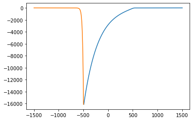
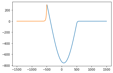
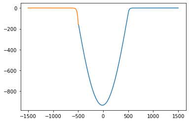
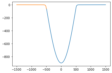
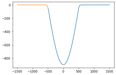
print(E)
plt.plot(Rwf_x, Rwf_y)
plt.plot(Lwf_x, Lwf_y)
plt.show()
for count in range(0, count_max + 1):
# Iteration loop
E = (Emax + Emin) / 2 # Divide E range
Diff = diff(E, h)
if diff(Emax, h) * Diff > 0:
Emax = E # Bisection algor
else:
Emin = E
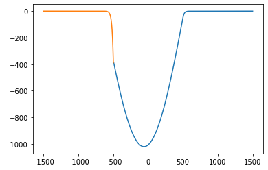
if abs(Diff) < eps:
break
plot(E, h)
print("Final eigenvalue E = ", E)
print("iterations, max = ", count)


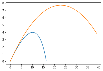
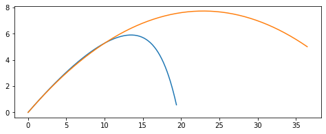
Problem 2: Projectile motion with drag
We can select a power $n=1$ or $2$. The friction coefficient is $k$.
$$ \ddot{x} = - k \dot{x}^n \frac{\dot{x}}{v} \\ \ddot{y} = - g - k \dot{y}^n \frac{\dot{y}}{v} \\ v = \sqrt{\dot{x}^2 + \dot{y}^2} $$We can rewrite it:
$$ u = \left(\begin{matrix} x \\ \dot{x} \\ y \\ \dot{y} \end{matrix}\right) $$Then:
$$ \dot{u} = \left(\begin{matrix} \dot{x} \\ - k \dot{x}^n \frac{\dot{x}}{v} \\ \dot{y} \\ - g - k \dot{y}^n \frac{\dot{y}}{v} \end{matrix}\right) = \left(\begin{matrix} u_1 \\ - k u_1^n \frac{u_1}{\sqrt{u_1^2 + u_3^2}} \\ u_3 \\ - g - k u_3^n \frac{u_3}{\sqrt{u_1^2 + u_3^2}} \end{matrix}\right) $$We can set the initial positions to 0 and give it a starting velocity, and compare no friction to friction versions.
import scipy.integrate
v0 = 22
angle = 34
g = 9.8
k = 0.8
n = 1

v0x = v0 * np.cos(np.radians(angle))
v0y = v0 * np.sin(np.radians(angle))

t_eval = np.linspace(0, 2)
analytic_x = v0x * t_eval
analytic_y = v0y * t_eval - 0.5 * g * t_eval ** 2
def f(t, u):
    v = np.sqrt(u[1] ** 2 + u[3] ** 2)
    return np.stack(
        [u[1], -k * u[1] ** n * u[1] / v, u[3], -g - k * u[3] ** n * u[3] / v]
    )
res = scipy.integrate.solve_ivp(f, [0, 2], [0, v0x, 0, v0y], t_eval=t_eval)
print(res.message)
plt.figure(figsize=(8, 3))
plt.plot(res.y[0], res.y[2])
plt.plot(analytic_x, analytic_y)
""" From "COMPUTATIONAL PHYSICS" & "COMPUTER PROBLEMS in PHYSICS"
    by RH Landau, MJ Paez, and CC Bordeianu (deceased)
    Copyright R Landau, Oregon State Unv, MJ Paez, Univ Antioquia,
    C Bordeianu, Univ Bucharest, 2017.
    Please respect copyright & acknowledge our work."""

# ProjectileAir.py: Order dt^2 projectile trajectory + drag

import numpy as np
import matplotlib.pyplot as plt

v0 = 22
angle = 34.0
g = 9.8
kf = 0.8
N = 20

v0x = v0 * np.cos(angle * np.pi / 180)
v0y = v0 * np.sin(angle * np.pi / 180)
T = 2 * v0y / g
H = v0y ** 2 / 2 / g
R = 2 * v0x * v0y / g

print("No Drag T =", T, ", H =", H, ", R =", R)


def plotNumeric(k):
    vx = v0 * np.cos(angle * np.pi / 180)
    vy = v0 * np.sin(angle * np.pi / 180)
    x = 0.0
    y = 0.0
    dt = vy / g / N * 1.5

    print("\n       With Friction  ")
    print("       x            y")

    xy = np.empty((2, N))
    xy[:, 0] = 0, 0

    for i in range(N - 1):
        vx = vx - k * vx * dt
        vy = vy - g * dt - k * vy * dt
        x = x + vx * dt
        y = y + vy * dt
        xy[:, i + 1] = x, y
        print(" %13.10f  %13.10f " % (x, y))

    plt.plot(*xy)


def plotAnalytic():
    v0x = v0 * np.cos(angle * np.pi / 180)
    v0y = v0 * np.sin(angle * np.pi / 180)
    dt = v0y / g / N * 1.8
    print("\n       No Friction  ")
    print("        x            y")

    xy = np.empty((2, N))
    for i in range(N):
        t = i * dt
        x = v0x * t
        y = v0y * t - g * t * t / 2
        xy[:, i] = x, y
        print(" %13.10f  %13.10f" % (x, y))

    plt.plot(*xy)


plotNumeric(kf)
plotAnalytic()