Monte Carlo Integration

Week 5 day 2: MC Integration

Objectives:

Become familiar with 2D arrays
Learn MC integration techniques

import numpy as np
import matplotlib.pyplot as plt

2D arrays

Most of the array creation routines take lists or tuples for size:

np.zeros((2, 3))

array([[0., 0., 0.],
       [0., 0., 0.]])

You can also use nested lists or arrays to the normal constructor:

m = np.array([[1, 2], [3, 4]])
print(m)

[[1 2]
 [3 4]]

print(m[0, :], "==", m[0])

[1 2] == [1 2]

m[:, 0]

array([1, 3])

np.sum(m, axis=1)

array([3, 7])

np.sum(m, axis=1, keepdims=True)

array([[3],
       [7]])

Area of a circle

$$ x^2 + y^2 \le 1 $$

xy = np.random.rand(2, 10000) * 2 - 1
valid = np.sum(xy ** 2, axis=0) < 1
good = xy[:, valid]
bad = xy[:, ~valid]

plt.plot(*good, ".")
plt.plot(*bad, ".")
plt.axis("equal")

(-1.0999373004325848,
 1.099984558528224,
 -1.0996322779437848,
 1.099814818306315)

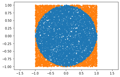
np.mean(valid) * 4

3.1536

Volume of a sphere:

xy = np.random.rand(2, 100000) * 2 - 1
r2 = np.sum(xy ** 2, axis=0)
r2[r2 > 1] = 1
print("MC:    ", np.mean(np.sqrt(1 - r2)) * 4 * 2)
print("Actual:", 4 / 3 * np.pi)

MC:     4.186083158623857
Actual: 4.1887902047863905

10 D example

$$ f(x) = \left(x_{1} + \cdots + x_{10}\right)^2 $$

def f(x):
    return np.sum(x, axis=0) ** 2

s = np.random.rand(10, 1000000)

np.mean(f(s))

25.826340350952517

155 / 6

25.833333333333332

Error estimate:

155 / 6 * 1 / np.sqrt(s.shape[1])

0.025833333333333333

Difficult functions to integrate

from scipy import stats

df = 2.74

begin, end = stats.t.cdf([-100, 100], df)
print("Analytic:", end - begin)

Analytic: 0.9999941949856226

x = np.linspace(-100, 100, 1_000)
fig, ax = plt.subplots()
ax.plot(x, stats.t.pdf(x, df))
plt.show()

X = (np.random.rand(1000) - 0.5) * 200
np.mean(stats.t.pdf(X, df)) * 200

1.0073131016541101

1 / np.sqrt(1000)

0.03162277660168379

Variance reduction

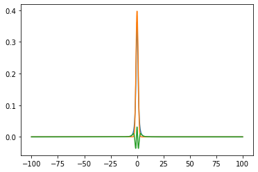
x = np.linspace(-100, 100, 1_000)
fig, ax = plt.subplots()
ax.plot(x, stats.t.pdf(x, df))
ax.plot(x, stats.norm.pdf(x, 0, 1))
ax.plot(x, stats.t.pdf(x, df) - stats.norm.pdf(x, 0, 1.2))
plt.show()

X = (np.random.rand(1000) - 0.5) * 200
Id = np.mean(stats.t.pdf(X, df) - stats.norm.pdf(X, 0, 1.2)) * 200
gaussInt = stats.norm.cdf(100, 0, 1.2) - stats.norm.cdf(-100, 0, 1.2)
print(Id + gaussInt)

1.0086732320144276

Importance sampling

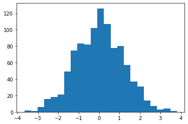
Xg = np.random.normal(0, 1.2, 1000)
Xg = Xg[np.abs(Xg) <= 10]
print(len(Xg))
np.mean(stats.t.pdf(Xg, df) / stats.norm.pdf(Xg, 0, 1.2))

0.9661111146296427

plt.hist(Xg, bins="auto")
plt.show()

Von Neumann Rejection

Xy = np.random.rand(2, 10000)
Xy[0] -= 0.5
Xy[0] *= 10

plt.plot(*Xy, ".")
plt.xlabel("x")
plt.ylabel("y")
plt.show()

w0 = 0.5  # Must be higher than the maximum of the PDF
Xy[1] *= w0

valid = Xy[1] < stats.t.pdf(Xy[0], df)

plt.plot(*Xy[:, valid], ".")
plt.plot(*Xy[:, ~valid], ".")
plt.xlabel("x")
plt.ylabel("y")
plt.show()

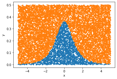
It's not a great way to calculate an integral, but we can:

np.mean(valid) * w0 * 10

0.9755