
21. Numba: JIT for Speed!#
Numba is one of the most exciting things to happen to Python. It is a library than take a Python function, convert the bytecode to LLVM, compile it, and run it at full machine speed!
import numba
import numpy as np
import matplotlib.pyplot as plt
21.1. First example#
def f1(a, b):
    return 2 * a**3 + 3 * b**0.5


@numba.vectorize
def f2(a, b):
    return 2 * a**3 + 3 * b**0.5
a, b = np.random.random_sample(size=(2, 100_000))
%%timeit
c = f1(a, b)
1.68 ms ± 5.94 μs per loop (mean ± std. dev. of 7 runs, 1,000 loops each)
%%time
c = f2(a, b)
CPU times: user 328 ms, sys: 11 ms, total: 339 ms
Wall time: 339 ms
This probably took a bit longer. The very first time you JIT compile something, it takes time to do the compilation. Numba is pretty fast, but you probably still pay a cost. There are things you can do to control when this happens, but there is a small cost.
%%timeit
c = f2(a, b)
73.8 μs ± 79.7 ns per loop (mean ± std. dev. of 7 runs, 10,000 loops each)
It took the function we defined, pulled it apart, and turned into Low Level Virtual Machine (LLVM) code, and compiled it. No special strings or special syntax; it is just a (large) subset of Python and NumPy. And users and libraries can extend it too. It also supports:
Vectorized, general vectorized, or regular functions
Ahead of time compilation, JIT, or dynamic JIT
Parallelized targets
GPU targets via CUDA or ROCm
Nesting
Creating cfunction callbacks
It is almost always as fast or faster than any other compiled solution (minus the JIT time). A couple of years ago it became much easier to install (via PIP with LLVMLite’s lightweight and independent LLVM build).
21.2. JIT example#
The example above using @numba.vectorize to make “ufunc” like functions. These can take any (broadcastable) size of array(s) and produces an output array. It’s similar to @numpy.vectorize which just loops in Python. Let’s try controlling the looping ourselves, using a ODE solver:
21.2.1. Problem setup#
Let’s setup an ODE function to solve. We can write our ODE as a system of linear first order ODE equations:
The harmonic motion equation can be written in terms of \(\mathbf{f}(t, \mathbf{y}) = \dot{\mathbf{y}}\), where this is in the standard form:
x_max = 1  # Size of x max
v_0 = 0
koverm = 1  # k / m


def f(t, y):
    "Y has two elements, x and v"
    return np.array([-koverm * y[1], y[0]])
21.2.2. Runge-Kutta introduction#
Note that \(h = t_{n+1} - t_n \).
Now, expand \(f\) in a Taylor series around the midpoint of the interval:
The second term here is symmetric in the interval, so all we have left is the first term in the integral:
Back into the original statement, we get:
We’ve got one more problem! How do we calculate \(f(t_{n+\frac{1}{2}},y_{n+\frac{1}{2}})\)? We can use the Euler’s algorithm that we saw last time:
Putting it together, this is our RK2 algorithm:
We’ve picked up bold face to indicate that we can have a vector of ODEs.
We can get the RK4 algorithm by keeping another non-zero term in the Taylor series:
def rk4_ivp(f, init_y, t):
    steps = len(t)
    order = len(init_y)

    y = np.empty((steps, order))
    y[0] = init_y

    for n in range(steps - 1):
        h = t[n + 1] - t[n]

        k1 = h * f(t[n], y[n])  # 2.1
        k2 = h * f(t[n] + h / 2, y[n] + k1 / 2)  # 2.2
        k3 = h * f(t[n] + h / 2, y[n] + k2 / 2)  # 2.3
        k4 = h * f(t[n] + h, y[n] + k3)  # 2.4

        y[n + 1] = y[n] + 1 / 6 * (k1 + 2 * k2 + 2 * k3 + k4)  # 2.0

    return y
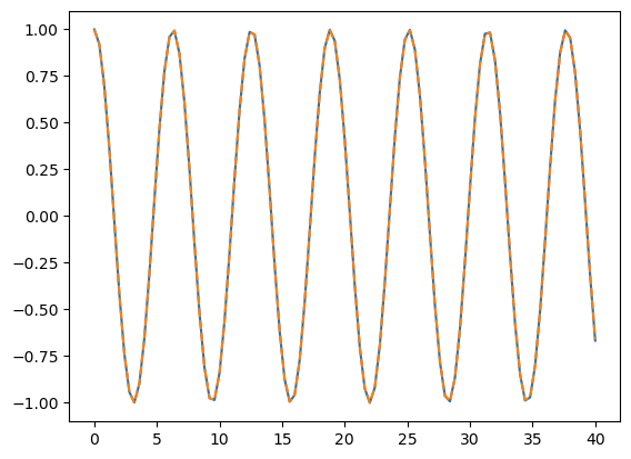
Let’s plot this:
ts = np.linspace(0, 40, 100 + 1)
y = rk4_ivp(f, [x_max, v_0], ts)
plt.plot(ts, np.cos(ts))
plt.plot(ts, y[:, 0], "--");
%%timeit
ts = np.linspace(0, 40, 1000 + 1)
y = rk4_ivp(f, [x_max, v_0], ts)
17.1 ms ± 65.1 μs per loop (mean ± std. dev. of 7 runs, 100 loops each)
21.2.3. Adding Numba#
Normally, you’d use a decorator here, but I’m lazy and don’t want to rewrite the function, so I’ll just manually apply the decorator, since we covered what the syntax actually does.
f_jit = numba.njit(f)
rk4_ivp_jit = numba.njit(rk4_ivp)
%%timeit
ts = np.linspace(0, 40, 1000 + 1)
y = rk4_ivp_jit(f_jit, np.array([x_max, v_0]), ts)
339 μs ± 61.1 μs per loop (mean ± std. dev. of 7 runs, 1 loop each)
You can inspect the types if you’d like to add them after running once:
f_jit.inspect_types()
f (float64, Array(float64, 1, 'C', False, aligned=True))
--------------------------------------------------------------------------------
# File: /tmp/ipykernel_4169/396120679.py
# --- LINE 6 ---
# label 0
#   t = arg(0, name=t)  :: float64
#   del t
#   y = arg(1, name=y)  :: array(float64, 1d, C)

def f(t, y):

    # --- LINE 7 ---

    "Y has two elements, x and v"

    # --- LINE 8 ---
    #   $4load_global.0 = global(np: <module 'numpy' from '/home/runner/work/level-up-your-python/level-up-your-python/.pixi/envs/default/lib/python3.13/site-packages/numpy/__init__.py'>)  :: Module(<module 'numpy' from '/home/runner/work/level-up-your-python/level-up-your-python/.pixi/envs/default/lib/python3.13/site-packages/numpy/__init__.py'>)
    #   $14load_attr.1 = getattr(value=$4load_global.0, attr=array)  :: Function(<built-in function array>)
    #   del $4load_global.0
    #   del $14load_attr.1
    #   $34load_global.3 = global(koverm: 1)  :: Literal[int](1)
    #   $44unary_negative.4 = unary(fn=<built-in function neg>, value=$34load_global.3)  :: int64
    #   del $34load_global.3
    #   $const48.6.1 = const(int, 1)  :: Literal[int](1)
    #   $50binary_subscr.7 = static_getitem(value=y, index=1, index_var=$const48.6.1, fn=<built-in function getitem>)  :: float64
    #   del $const48.6.1
    #   $binop_mul54.8 = $44unary_negative.4 * $50binary_subscr.7  :: float64
    #   del $50binary_subscr.7
    #   del $44unary_negative.4
    #   $const60.10.2 = const(int, 0)  :: Literal[int](0)
    #   $62binary_subscr.11 = static_getitem(value=y, index=0, index_var=$const60.10.2, fn=<built-in function getitem>)  :: float64
    #   del y
    #   del $const60.10.2
    #   size = const(int, 2)  :: int64
    #   size_tuple = build_tuple(items=[Var(size, 396120679.py:8)])  :: UniTuple(int64 x 1)
    #   del size_tuple
    #   empty_func = global(empty: <built-in function empty>)  :: Function(<built-in function empty>)
    #   $np_g_var = global(np: <module 'numpy' from '/home/runner/work/level-up-your-python/level-up-your-python/.pixi/envs/default/lib/python3.13/site-packages/numpy/__init__.py'>)  :: Module(<module 'numpy' from '/home/runner/work/level-up-your-python/level-up-your-python/.pixi/envs/default/lib/python3.13/site-packages/numpy/__init__.py'>)
    #   $np_typ_var = getattr(value=$np_g_var, attr=float64)  :: dtype(float64)
    #   del $np_g_var
    #   $68call.13 = call empty_func(size, $np_typ_var, func=empty_func, args=[Var(size, 396120679.py:8), Var($np_typ_var, 396120679.py:8)], kws={}, vararg=None, varkwarg=None, target=None)  :: (int64, dtype(float64)) -> array(float64, 1d, C)
    #   del size
    #   del empty_func
    #   del $np_typ_var
    #   index = const(int, 0)  :: int64
    #   $68call.13[index] = $binop_mul54.8  :: (Array(float64, 1, 'C', False, aligned=True), int64, float64) -> none
    #   del index
    #   del $binop_mul54.8
    #   index.1 = const(int, 1)  :: int64
    #   $68call.13[index.1] = $62binary_subscr.11  :: (Array(float64, 1, 'C', False, aligned=True), int64, float64) -> none
    #   del index.1
    #   del $62binary_subscr.11
    #   $76return_value.14 = cast(value=$68call.13)  :: array(float64, 1d, C)
    #   del $68call.13
    #   return $76return_value.14

    return np.array([-koverm * y[1], y[0]])


================================================================================