
19. NumPy: Numeric computing#
The core of all modern scientific computing. You should know this one! This is NumPy + SciPy + Matplotlib, which form the core of the modern computing stack for Scientific Python.
import numpy as np
import matplotlib.pyplot as plt
It is used for N-dimensional arrays:
v = np.array([1, 2, 3])
v
array([1, 2, 3])
The clever trick is that computations on an array are pre-compiled, and can be much faster than Python:
v**2
array([1, 4, 9])
Note that it was designed for large arrays; around 10 elements or less you might be faster using plain Python (though it’s still more expressive). You should “vectorize” your code (by making the arrays bigger with more dimensions) if your arrays are very small and you care about performance.
In the spirit of the course, I’ll avoid covering the basics of NumPy here (arrays, simple dtypes, operations), and instead focus on intermediate features.
19.1. Slicing#
NumPy slicing may not make copies of arrays, but can just adjust the start and strides of the data. This is usually true of reshaping and adding empty (length 1) dimensions, as well. For example:
arr = np.zeros([2, 3, 4], dtype=int)
print(arr.flags)
  C_CONTIGUOUS : True
  F_CONTIGUOUS : False
  OWNDATA : True
  WRITEABLE : True
  ALIGNED : True
  WRITEBACKIFCOPY : False
Slicing produces a copy; we can see the effect of setting values, for example:
x = arr[:, :2, 2:]
x[...] = 1
print(arr)
[[[0 0 1 1]
  [0 0 1 1]
  [0 0 0 0]]

 [[0 0 1 1]
  [0 0 1 1]
  [0 0 0 0]]]
Flattening also avoids a copy if the data is contagious:
y = arr.ravel()
y[:3] = 2
print(arr)
[[[2 2 2 1]
  [0 0 1 1]
  [0 0 0 0]]

 [[0 0 1 1]
  [0 0 1 1]
  [0 0 0 0]]]
However, flattening / reshaping an array without a copy may not always be possible, such as if the data is non-contagious:
y = arr.T.ravel()
y[:3] = 3
print(arr)
[[[2 2 2 1]
  [0 0 1 1]
  [0 0 0 0]]

 [[0 0 1 1]
  [0 0 1 1]
  [0 0 0 0]]]
19.2. Random Numbers#
The simple random number interface np.random.<distribution> should only be used for highly interactive work. Normal usage should use a more modern, object oriented approach; first construct a random number generator:
rng = np.random.default_rng()
You can pass an explicit seed if you want reproducibility. Then this generator has distributions as methods:
dist = rng.normal(0, 1, size=1_000_000)
fix, ax = plt.subplots()
ax.hist(dist, bins=100)
plt.show()

The benefits include explicit control over the generator, reproducibility, and support for multiple independent generators.
19.3. Broadcasting#
One benefit of true 1D arrays (vs. languages that don’t have 1D arrays) is that NumPy can support broadcasting. Broadcasting occurs whenever an operation (element-wise or matrix multiplication) encounters an array that is the wrong shape. The rules can be viewed two ways:
If the number of dimensions does not match, prepend length-1 dimensions until they do.
If the size of a dimension does not match and one of the dimensions is 1, duplicate along that axis to make it match.
Or:
Moving right to left, if a dimension is missing or 1, set the stride to 0 on that array, so the iteration pointer does not change along that dimension.
The former is often easier to reason about, while the later is how it’s implemented (so it is very efficient).
(np.ones((2, 3, 4)) * np.ones((1, 4))).shape
(2, 3, 4)
You can predict the final shape with broadcast_shapes:
np.broadcast_shapes((2, 3, 4), (1, 4))
(2, 3, 4)
You can also explicitly expand with np.broadcast_arrays.
Broadcasting is extremely useful for array-at-a-time programming, such as for coordinate arrays and the like. If you organize your calculations to delay expansion, you can optimize a lot of computation out.
For example, we can use ogrid or meshgrid(..., sparse=True) to replace mgrid but with compressed arrays ready for broadcasting. Here we make a grid with 101 points on x from 1-2 and 501 points on y from 0 to 5 (ends inclusive):
x, y = np.mgrid[2.5:3.5:101j, 0:5:501j]
radius = np.sqrt(x**2 + y**2)
print(f"{x.shape=}, {y.shape=}")
print(f"{radius[50,400] = }")
x.shape=(101, 501), y.shape=(101, 501)
radius[50,400] = np.float64(5.0)
x, y = np.ogrid[2.5:3.5:101j, 0:5:501j]
radius = np.sqrt(x**2 + y**2)
print(f"{x.shape=}, {y.shape=}")
print(f"{radius[50,400] = }")
x.shape=(101, 1), y.shape=(1, 501)
radius[50,400] = np.float64(5.0)
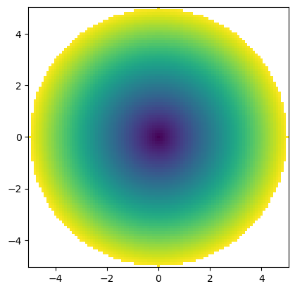
19.4. Masked arrays#
A powerful and under supported feature is masked arrays. If values are missing, you can “mask” them.
This is quite nice logically, but the downside is not all interfaces support masked arrays. You also use extra space for the boolean mask. Another trick is to use NaN’s in a floating point array, or to use Pandas’s support for None’s in all arrays.
x, y = np.mgrid[-5:5:101j, -5:5:101j]
radius = np.sqrt(x**2 + y**2)
mradius = np.ma.masked_where(radius > 5, radius)
fix, ax = plt.subplots()
ax.pcolormesh(x, y, mradius)
ax.set_aspect("equal")
plt.show()
19.5. Record arrays (AKA preview for Pandas!)#
NumPy has support for complex DTypes. While Pandas or xarray handles structured dtypes more elegantly (and in a columnar form), but if you actually have data from some source that is structured and in an array form, this can be incredibly useful.
arr = np.array([(1, 2.0), (3, 4.0)], dtype=[("id", int), ("val", float)])
arr
array([(1, 2.), (3, 4.)], dtype=[('id', '<i8'), ('val', '<f8')])
You can select out a single named dtype (without copy) as well:
arr["val"]
array([2., 4.])
19.6. Smaller features#
19.6.1. Buffer protocol#
There’s a buffer protocol in Python 3 that allows different libraries to communicate this sort of data without copies. This is also useful to communicate things like shared memory or existing memory to NumPy.
import array
python_array = array.array("d", (1, 2, 3, 4))
We can explicitly convert from a buffer:
np.frombuffer(python_array)
array([1., 2., 3., 4.])
Or most NumPy functions also work directly on buffers by converting them:
arr = np.asarray(python_array)
This “conversion” does not copy! You still are looking at the buffer’s original memory:
arr[1] = 42
python_array
array('d', [1.0, 42.0, 3.0, 4.0])
You can verify that the NumPy array doesn’t own the memory:
arr.flags.owndata
False
19.7. Custom arrays#
19.7.1. UFuncs#
NumPy has the concept of UFuncs; functions that can take array arguments (broadcastable) and will return a broadcast result. For example:
np.sin(1)
np.float64(0.8414709848078965)
np.sin(np.array([0, 1, 2]))
array([0. , 0.84147098, 0.90929743])
np.add(7, np.arange(3))
array([7, 8, 9])
UFuncs have several standard keyword arguments:
out: Output to existing array, skip allocationwhere: Mask computationaxes,axis: axes to operate on (generalized UFuncs only)keepdims: To remove reduced dims (some generalized UFuncts only)casting='same_kind': rules for casting different DTypesorder='K': memory layout (“K”eep)dtype=None: Dtype for output arraysubok=True: Output can be a subclasssignature/extobj: Exact control over dtypes/buffers
(A generalized UFunc supports specific patterns, like matrix multiplication, rather than being element-wise)
UFuncs also support several methods and have a few properties. There are exactly six methods:
__call__: Elementwise computationat: Local elementwise computation (provide indices)reduce: A reductionreduceat: A local reduction (provide indices)accumulate: An accumulationouter: An outer apply (np.multiply.outeris identical tonp.tensordot)
19.7.2. NEP 13/18#
If you have a custom class, you can also customize UFuncs via NEP 13!
# Aside: let's add pytest's raises decorator
import pytest
class SimpleUnc(np.ndarray):
    pass


def simple_unc(val, unc):
    arr = np.array(list(zip(val, unc)), dtype=[("val", float), ("unc", float)])
    return arr.view(SimpleUnc)
a = simple_unc([1, 2, 3], [0.1, 0.1, 0.1])
a
SimpleUnc([(1., 0.1), (2., 0.1), (3., 0.1)],
          dtype=[('val', '<f8'), ('unc', '<f8')])
a == a
SimpleUnc([ True, True, True])
We can see that this does raise an error if you try to add it, though:
with pytest.raises(TypeError):
    a + a
Now let’s provide __array_ufunc__, which will allow us to customize the behavior of UFuncs. This will use Python 3.10’s pattern matching for simplicity.
class SimpleUnc(np.ndarray):
    def __array_ufunc__(self, ufunc, method: str, *inputs, **kwargs):
        # Avoid infinite recursion
        raw_inputs = [np.asarray(x) for x in inputs]

        match (ufunc, method, raw_inputs):
            # Custom add / subtract
            case np.add | np.subtract, "__call__", (a, b):
                # This can waste an allocation
                (result,) = kwargs.pop("out", [np.empty(self.shape, self.dtype)])

                ufunc(a["val"], b["val"], out=result["val"], **kwargs)
                np.add(a["unc"] ** 2, b["unc"] ** 2, out=result["unc"], **kwargs)
                np.sqrt(result["unc"], out=result["unc"], **kwargs)

                return result.view(self.__class__)

            # Fall back on whatever it would have done before - do not return this subclass
            case _:
                return super().__array_ufunc__(ufunc, method, *raw_inputs, **kwargs)
a = simple_unc([1, 2, 3], [0.1, 0.1, 0.1])
a + a
SimpleUnc([(2., 0.14142136), (4., 0.14142136), (6., 0.14142136)],
          dtype=[('val', '<f8'), ('unc', '<f8')])
a - a
SimpleUnc([(0., 0.14142136), (0., 0.14142136), (0., 0.14142136)],
          dtype=[('val', '<f8'), ('unc', '<f8')])
This is very simple and doesn’t account for correlations, but it does show that it works.
a == a
array([ True, True, True])
There’s a lot more to NumPy; it’s worth looking around in the docs. An example of a function you might find is np.diff(a), which is equivalent to a[:-1] - a[1:] but reads better without repeating the array name. Also look at the huge number of useful methods in SciPy.