Week 9 Day 1: Confidence intervals

Objectives:

Look at sampling confidence intervals
Look at frequentist confidence intervals

Confidence intervals example

Based loosely on A very friendly introduction to confidence intervals

import numpy as np
import scipy.stats as stats
import matplotlib.pyplot as plt

Let's look at taking a small sample of a larger distribution. We'll use the same example given in the reference; this was a poll of the people in the US to see what fraction likes Soccer. Let's assume for the moment we know the real mean, and have the original distribution handy:

love_soccer_prop = 0.65  # Real percentage of people who love soccer
total_population = 325*10**6  # Total population in the U.S. (325M)
# Note: 325e6 would be a floating point number

love_soccer_num = int(love_soccer_prop * total_population)

Bools are smaller than ints, and we can still take the mean, sum, etc. of an array of bools, so we'll use bools. We'll start off with a "sorted" array (people who love Soccer first), we we'll need to be careful when we select samples from it.

population = np.zeros(total_population, dtype=bool)
population[:love_soccer_num] = True

np.mean(population)

0.65

for i in range(10):
    sample = np.random.choice(population, size=1000)
    print(f'Sample {i}: {np.mean(sample)}')

Sample 0: 0.618
Sample 1: 0.669
Sample 2: 0.64
Sample 3: 0.651
Sample 4: 0.66
Sample 5: 0.668
Sample 6: 0.674
Sample 7: 0.656
Sample 8: 0.629
Sample 9: 0.664

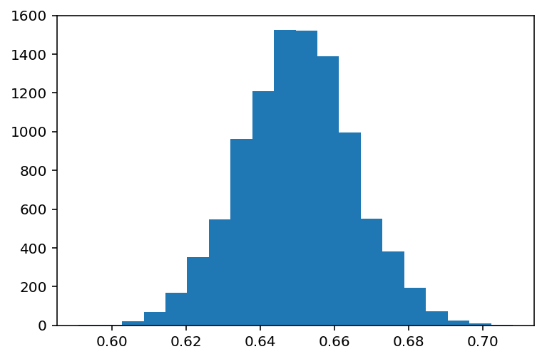
values = np.empty(10_000)
for i in range(len(values)):
    values[i] = np.mean(np.random.choice(population, size=1_000))

np.mean(values)

0.6499228000000001

plt.hist(values, bins=20)
plt.show()

confidence=0.95
sem = np.std(sample) / np.sqrt(len(sample)) # scipy.stats.sem(sample)
h = sem * scipy.stats.t.ppf((1 + confidence) / 2, len(sample)-1)
print(f"{np.mean(sample)} +/- {h:.3g} ({confidence:.1%})")

0.664 +/- 0.0293 (95.0%)

For larger samples (more than 100), we can approximate the student's t distribution with a Gaussian:

sem = scipy.stats.sem(sample)
h = sem * scipy.stats.norm.ppf((1 + confidence) / 2)
print(f"{np.mean(sample)} +/- {h:.3g} ({confidence:.1%})")

0.664 +/- 0.0293 (95.0%)

In SciPy, we can do this even quicker:

h = scipy.stats.t.interval(confidence, len(sample)-1, loc=np.mean(sample), scale=sem)
print(h)

(0.6346744940182318, 0.6933255059817682)

Anaconda includes another popular package for statistics: StatsModels, which complements scipy.stats and pandas.

import statsmodels.stats.api as sms

inter = sms.DescrStatsW(sample).tconfint_mean()
inter

(0.6346744940182318, 0.6933255059817682)

Physics confidence intervals

Based on the excellent slides here: http://www.phas.ubc.ca/~oser/p509/Lec_16.pdf

For simplicity, we will assume that we are using 90% confidence intervals in the notes below.

In Physics, frequentist confidence intervals are often used for measurements. We make a measurement, then construct a confidence interval from the expected underlying probability distribution for the different possible measurements; we quote the true values for which our measurement is in the 90% range.

This does not tell us that there is a 90% chance the true value is in this range, rather that if we did this experiment many times, 90% of the experiments would contain the true value.

Neyman confidence interval construction:

Calculate the PDF of obtaining a measurement $\hat{a}$ from the true value $a$: $\mathrm{P}(\hat{a}|a)$
Define the interval where $\hat{a}$ has a 90% chance of occurring
Repeat for all possible true $a$

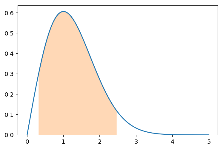
If we have the following distribution, the Neyman confidence interval construction does not specify how to draw the confidence region; any region that contains 90% of the probability could be a 90% confidence interval.

$$ \mathrm{PDF}(x) = x e^{-\frac{1}{2} x^2} $$

import sympy as s
s.init_printing()

x = s.symbols('x')
f = x * s.exp(-x**2/2)

f.integrate(x)

$$- e^{- \frac{x^{2}}{2}}$$

This is normalized:

f.integrate((x,0,s.oo))

$$1$$

This is one region:

f.integrate((x,0.32,2.45))

$$0.900363760390277$$

fn = s.lambdify([x], f)

xs = np.linspace(0,5,100)
plt.plot(xs,fn(xs))
xs = np.linspace(0.32,2.45,50)
plt.fill_between(xs, fn(xs), color='C1', alpha=.3)
plt.ylim(ymin=0)
plt.show()

You can also choose an upper limit:

f.integrate((x,0,2.15))

$$0.900862747489253$$

xs = np.linspace(0,5,100)
plt.plot(xs,fn(xs))
xs = np.linspace(0,2.15,50)
plt.fill_between(xs, fn(xs), color='C1', alpha=.3)
plt.ylim(ymin=0)
plt.show()

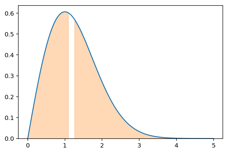
How about this?

f.integrate((x,0,1.09)) + f.integrate((x,1.26,s.oo))

$$0.900036658396236$$

xs = np.linspace(0,5,100)
plt.plot(xs,fn(xs))
xs = np.linspace(0,1.09,50)
plt.fill_between(xs, fn(xs), color='C1', alpha=.3)
xs = np.linspace(1.26,5,50)
plt.fill_between(xs, fn(xs), color='C1', alpha=.3)
plt.ylim(ymin=0)
plt.show()

Flip flop problem

Let's take the following example. Assume I am measuring from a Gaussian distribution where I know $\mu\ge0$:

$$ \mathrm{P}(\hat{\mu} | \mu) = \frac{1}{\sqrt{2\pi}} \exp{\left[ -\frac{1}{2} \left( \mu - \hat{\mu} \right)^2 \right]} $$

For fixed true value $\mu$, 90% of the probability lies in $\mu-1.28<\hat{\mu}<\infty$. Or $\mu-1.65<\hat{\mu}<\mu+1.65$.

fig, ax = plt.subplots()

# Upper limit quote
x = np.linspace(0,3)
ax.fill_between(x, 1.28 + x, alpha=.3)

# Upper and lower bounds
x = np.linspace(3,4)
ax.fill_between(x, 1.65 + x, x - 1.65, alpha=.3)

# Quote as 0
x = np.linspace(-2,0)
ax.fill_between(x, 1.28 + x*0, alpha=.3)

ax.set_xlim(-2,4)
ax.set_ylim(0,6)
ax.grid()
ax.set_aspect('equal')
plt.show()

Feldman-Cousins

A special prescription for building the limits intervals that transitions properly and avoids empty set when near a physical boundary (like 0) by using the following ordering ratio:

$$ R = \frac{P(x∣\mu)} {P(x∣\mu_\mathrm{best})} $$

You simply select the 90% with the highest R.

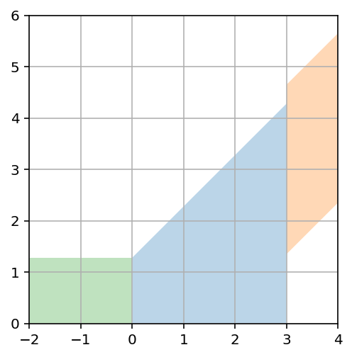
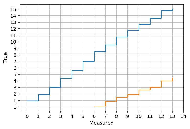
From out previous example, $\mu_\mathrm{best}=x$ if $x>0$ or $\mu_\mathrm{best}=0$ if $x\le 0$

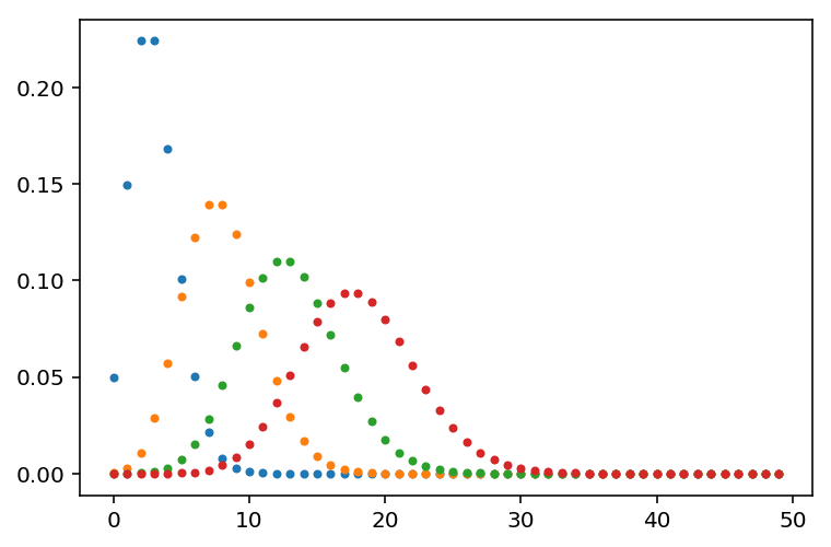
Feldman-cousins from GammaPy (from pip)

import gammapy.stats as gstats

x_bins = np.arange(0, 50)
mu_bins = np.linspace(0, 15, int(15/0.005) + 1, endpoint=True)
matrix = [stats.poisson(mu + 3.0).pmf(x_bins) for mu in mu_bins]

plt.plot(matrix[0], '.')
plt.plot(matrix[1000], '.')
plt.plot(matrix[2000], '.')
plt.plot(matrix[-1], '.')

[<matplotlib.lines.Line2D at 0x1a19712748>]

acceptance_intervals = gstats.fc_construct_acceptance_intervals_pdfs(matrix, 0.9)
LowerLimitNum, UpperLimitNum, other = gstats.fc_get_limits(mu_bins, x_bins, acceptance_intervals)

u = np.array([gstats.fc_find_limit(i, UpperLimitNum, mu_bins) for i in range(14)])
l = [gstats.fc_find_limit(i, LowerLimitNum, mu_bins) for i in range(14)]
plt.step(range(14), u, where='post', label='Upper limit')
plt.step(range(14), l, where='post', label='Lower limit')
plt.xticks(range(15))
plt.yticks(range(16))
plt.grid()
plt.xlabel('Measured')
plt.ylabel('True')
plt.show()